More Pandas DataFrame

In this article, we will explore the merge, the groupby, and the pivot_table functions of Pandas DataFrame.

Open a terminal window and fire off the IPython Notebook.

To begin using DataFrame, one must import the pandas module as shown below:

import numpy as np

import pandas as pd

Notice we have also imported numpy as we will be using it.

Just as one can perform a join (inner or outer) on two (or more) database tables in SQL, one can perform a similar join operation on Pandas DataFrame using the merge function.

Let us create two simple DataFrames called df1 and df2 to demostrate the merge function.

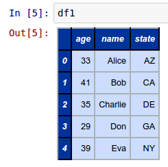
Create a simple 5 rows by 3 columns DataFrame called df1 as shown below:

df1 = pd.DataFrame({'name': ['Alice', 'Bob', 'Charlie', 'Don', 'Eva'], 'state': ['AZ', 'CA', 'DE', 'GA', 'NY'], 'age': [33, 41, 35, 29, 39]})

The following shows the screenshot of the result in IPython:

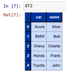
Next, create another simple 5 rows by 2 columns DataFrame called df2 as shown below:

df2 = pd.DataFrame({'name': ['Alice', 'Bob', 'Charlie', 'Frank', 'John'], 'car': ['Acura', 'BMW', 'Chevy', 'Honda', 'Toyota']})

The following shows the screenshot of the result in IPython:

To perform an inner join of the two DataFrames called df1 and df2, invoke the merge function as shown below:

The following shows the screenshot of the result in IPython:

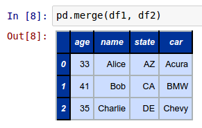
The merge function on two DataFrames defaults to an inner join operation.

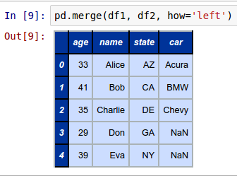
One can specify the how parameter on the merge function to control the type of join operation. If the how parameter equals left, an outer join is performed with the keys from the DataFrame on the left. If the how parameter equals right, an outer join is performed with the keys from the DataFrame on the right. And finally, if the how parameter equals outer, an outer join is performed with the union of keys from both the DataFrames.

To perform an outer join of the two DataFrames called df1 and df2 with the keys from the DataFrame on the left (df1), invoke the merge function as shown below:

The following shows the screenshot of the result in IPython:

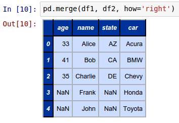
To perform an outer join of the two DataFrames called df1 and df2 with the keys from the DataFrame on the right (df2), invoke the merge function as shown below:

The following shows the screenshot of the result in IPython:

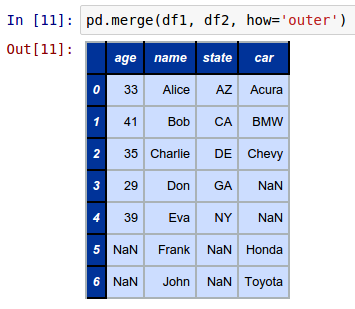
To perform an outer join of the two DataFrames called df1 and df2 with the union of keys from both the DataFrames (df1 and df2), invoke the merge function as shown below:

The following shows the screenshot of the result in IPython:

Just as one can perform aggregations (or transformations) on a database table in SQL using the group-by operation, one can perform similar aggregations (or transformations) on a Pandas DataFrame using the groupby function.

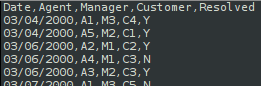
Let us create a fictitious call center activity dataset called call_center.csv.

The following shows the screenshot of the top few records from the dataset:

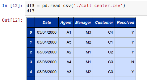
Create a DataFrame called df3 by loading the fictitious call center activity dataset as shown below:

The following shows the screenshot of the portion of the result from IPython:

To aggregate and display the total number of customer calls handled by each call center agent by manager from the above DataFrame called df3, invoke the groupby function as shown below:

The following shows the screenshot of the result in IPython:

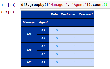
The groupby function uses a 3 step process called split-apply-combine to perform the desired operation. In the first step, the data is split into groups according to the specified column(s). In the second step, the specified aggregate (or transformation) operation such as count(), sum(), mean(), var(), std(), etc., is applied to each group. Finally, in the third step, the results are combined for the groups.

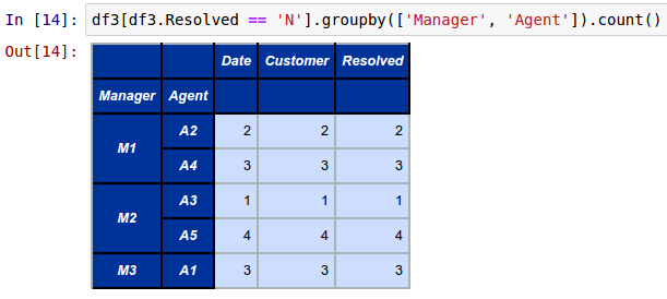
To aggregate and display the total number of un-resolved customer calls by each call center agent by manager from the above DataFrame called df3, invoke the groupby function as shown below:

df3[df3.Resolved == 'N'].groupby(['Manager', 'Agent']).count()

The following shows the screenshot of the result in IPython:

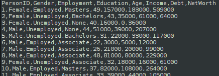
Now, let us create a fictitious household savings dataset called savings.csv.

The following shows the screenshot of the top few records from the dataset:

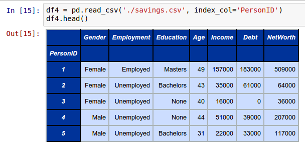
Create a DataFrame called df4 with PersonID as the index column by loading the fictitious household savings dataset as shown below:

df4 = pd.read_csv('./savings.csv', index_col='PersonID')

The following shows the screenshot of the portion of the result from IPython:

Let us create a groupby object called gdf1 from the above DataFrame called df4 by invoking the groupby function on the Education column as shown below:

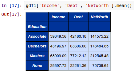
To compute and display the average (mean) Income, Debt, and NetWorth by Education from the above groupby object called gdf1, invoke the mean function as shown below:

The following shows the screenshot of the result in IPython:

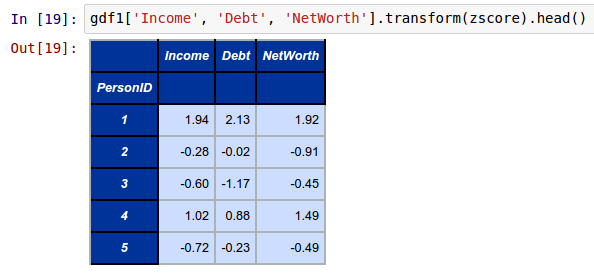
Now, let us define a function to compute the Z-Score of a numeric column.

Per Wikipedia, a Z-Score is a statistical measurement of a score's relationship to the mean in a group of scores. A Z-Score of 0 means the score is the same as the mean. A Z-Score can also be either positive or negative, indicating whether it is above or below the mean and by how many standard deviations.

The following lambda function defines how to compute the Z-Score of a numeric column:

To compute and display the Z-Score on numeric columns Income, Debt, and NetWorth by Education from the above groupby object called gdf1, invoke the transform function specifying the above zscore lambda as shown below:

gdf1['Income', 'Debt', 'NetWorth'].transform(zscore).head()

The following shows the screenshot of the result in IPython:

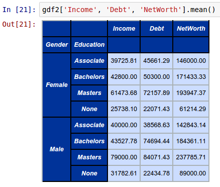
Now, let us create a groupby object called gdf2 from the above DataFrame called df4 by invoking the groupby function on the Gender and the Education columns as shown below:

To compute and display the average (mean) Income, Debt, and NetWorth by Gender and Education from the above groupby object called gdf2, invoke the mean function as shown below:

The following shows the screenshot of the result in IPython:

To compute and display the standard deviation of Income, Debt, and NetWorth by Gender and Education from the above groupby object called gdf2, invoke the std function as shown below:

The following shows the screenshot of the result in IPython:

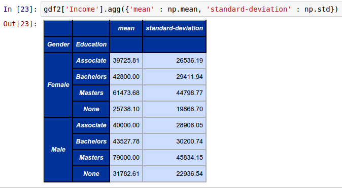
To compute and display both the mean and standard deviation of Income, Debt, and NetWorth by Gender and Education from the above groupby object called gdf2, invoke the agg function by passing a dictionary of the mean() and std() operations as shown below:

gdf2['Income'].agg({'mean' : np.mean, 'standard-deviation' : np.std})

The following shows the screenshot of the result in IPython:

Often times we want to slice and dice a given tabular data into a different view. For example, given our household savings dataset, we may want a view of the averages (mean) NetWorth for different Employment types across different Education levels.

The following shows the screenshot of the desired view from the original household savings view:

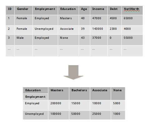
This is where the Pivot tables come into play. Pivot tables are created from a given DataFrame using the pivot_table function.

To create a Pivot table of averages (mean) NetWorth for different Education levels (columns) for each Employment type (rows) from the above DataFrame called df4, invoke the pivot_table function as shown below:

df4.pivot_table(index='Employment', columns='Education', values='NetWorth')

The following shows the screenshot of the result from IPython:

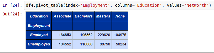
The pivot_table function takes 3 parameters - index (which indicates the keys of the pivot), columns of the pivot, and values (columns to aggregate on).

By default, the pivot_table function uses np.mean() for the aggregation operation.

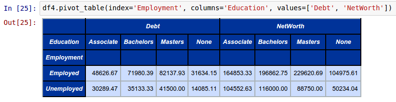
To create a Pivot table of averages (mean) for both Debt and NetWorth for different Education levels (columns) for each Employment type (rows) from the above DataFrame called df4, invoke the pivot_table function as shown below:

df4.pivot_table(index='Employment', columns='Education', values=['Debt', 'NetWorth'])

The following shows the screenshot of the result from IPython:

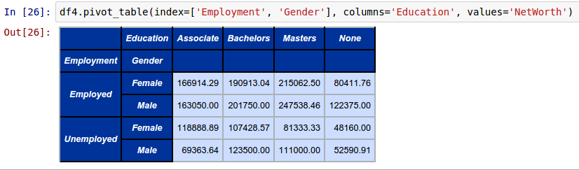
To create a Pivot table of averages (mean) NetWorth for different Education levels (columns) for each Employment and Gender comnination (rows) from the above DataFrame called df4, invoke the pivot_table function as shown below:

df4.pivot_table(index=['Employment', 'Gender'], columns='Education', values='NetWorth')

The following shows the screenshot of the result from IPython:

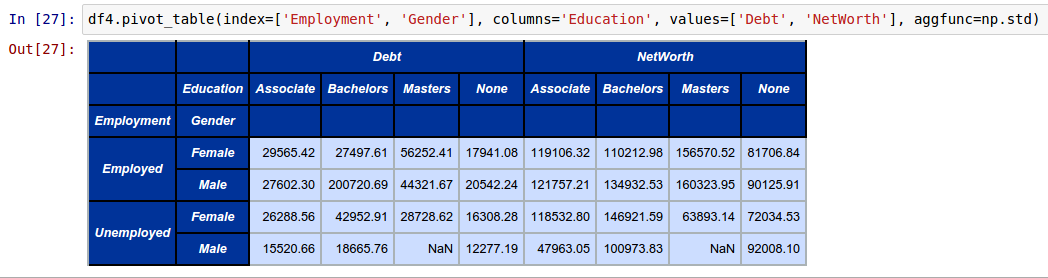
To create a Pivot table of standard deviations for both Debt and NetWorth for different Education levels (columns) for each Employment and Gender comnination (rows) from the above DataFrame called df4, invoke the pivot_table function by specifying the additional aggfunc as shown below:

df4.pivot_table(index=['Employment', 'Gender'], columns='Education', values=['Debt', 'NetWorth'], aggfunc=np.std)

The following shows the screenshot of the result from IPython: