Machine Learning - Logistic Regression - Part 1

Overview

Often times in the real world, the dependent outcome (or target) variable is NOT always a continuous random variable (quantitative), but a discrete random variable (qualitative or categorical). In such cases, the Linear Regression models do not work well and we will need a different approach. This is where the techniques of Classification come in handy. Classification is a statistical process, which attempts to segregate the observations from the dependent target (or a response) variable into one of the pre-determined set of categorical classes.

Logistic Regression is applicable when the Dependent Outcome (sometimes called a Response or a Target) variable $y$ is a dichotomous (or binary) CATEGORICAL variable and has some linear relationship with one or more of Independent Feature (or Predictor) variable(s) $x_1, x_2, ..., x_n$.

The value of the outcome (or target) variable $y$ is a binary - either a $0$ (referred to as a class $0$, a Failure, or a Negative) OR a $1$ (referred to as a class $1$, a Success, or a Positive).

Logistic Regression

In the following sections, we will use mathematical intuition to arrive at the Logistic Regression model.

We know there exists a linear relationship between the dependent target variable $y$ and the independent feature variables $x_1, x_2, ..., x_n$. This relationship can be expressed (using the matrix notation) as follows:

    $y = \beta_0 + \sum_{i=1}^n \beta_i x_i = X\beta$ ..... $\color{red} (1)$

where $X$ is the matrix of features and $\beta$ is the vector of coefficients.

Also, for Logistic Regression, the dependent outcome (or target) variable $y$ predicts the probability of a $1$ (referred to as a class $1$, a Success, or a Positive) or a $0$ (referred to as a class $0$, a Failure, or a Negative), based on the linear relationship with one or more independent feature variables $x_1, x_2, ..., x_n$. This implies that the range of the dependent target (or response) variable $y$ is in the range of $0$ to $1$.

We can rewrite the equation $\color{red} (1)$ from above as follows:

    $p(X) = X\beta$ ..... $\color{red} (2)$

where $p(X)$ is the probability for the dependent outcome (or target) variable $y$.

From the equation $\color{red} (2)$ above, it is clear that there is a mismatch between the right hand side and the left hand side of the equation. The right hand side is unbounded in the range $(-\infty, \infty)$, while the left hand side is bounded in the range $(0, 1)$.

From the concepts in probability, we know that if $p(X)$ is the probability of predicting a $1$ (or success), then the probability of predicting a $0$ (or failure) is $(1 - p(X))$.

Also, from probability, odds is expressed as a ratio of the probability of the event happening over the probability the event not happening. In other words:

    $odds = \Large{\frac{p(X)}{1-p(X)}}$ ..... $\color{red} (3)$

Let us now rewrite the equation $\color{red} (2)$ from above in terms of the equation $\color{red} (3)$ as follows:

    $\Large{\frac{p(X)}{1-p(X)}}$ $= X\beta$ ..... $\color{red} (4)$

From the equation $\color{red} (4)$ above, we still have a mismatch between the right hand side and the left hand side of the equation. The right hand side is unbounded in the range $(-\infty, \infty)$, while the left hand side is half-unbounded in the range $(0, \infty)$.

Let us now rewrite the equation $\color{red} (4)$ from above in terms of natural logarithm as follows:

    $\ln({\Large{\frac{p(X)}{1-p(X)}}})$ $= X\beta$ ..... $\color{red} (5)$

From the equation $\color{red} (5)$ above, as the probability $p(X)$ tends towards $1$, the natural log will tend towards $\infty$ and similarly as the probability $p(X)$ tends towards $0$, the natural log will tend towards $-\infty$. This means the left hand side is unbounded in the range $(-\infty, \infty)$ just like the right hand side of the equation.

Now that the left hand side and the right hand side match, let us now try to simplify the equation $\color{red} (5)$ from above.

*** Basic Rule of Natural Logarithm ***

  If $\ln(a) = b$, then $a = e^{b}$

Using the basic rule of logarithms, we can rewrite the equation $\color{red} (5)$ from above as follows:

    $\Large{\frac{p(X)}{1-p(X)}}$ $= e^{X\beta}$ ..... $\color{red} (6)$

Simplifying the the equation $\color{red} (6)$ from above, we get:

    $p(X) = (1 - p(X)).e^{X\beta}$

Expanding the right hand side, we get:

    $p(X) = e^{X\beta} - p(X)).e^{X\beta}$

Moving all the $p(X)$ terms together, we get:

    $p(X) + p(X)).e^{X\beta} = e^{X\beta}$

Pulling the common $p(X)$ term out, we get:

    $p(X).(1 + e^{X\beta}) = e^{X\beta}$

Simplifying the equation further, we get:

$\color{red} \boldsymbol{p(X)}$ $=$ $\bbox[pink,2pt]{\Large{\frac{e^{X\beta}}{1 + e^{X\beta}}}}$ $=$ $\bbox[pink,2pt] {\Large{\frac{1}{1 + e^{-X\beta}}}}$ ..... $\color{blue} (A)$

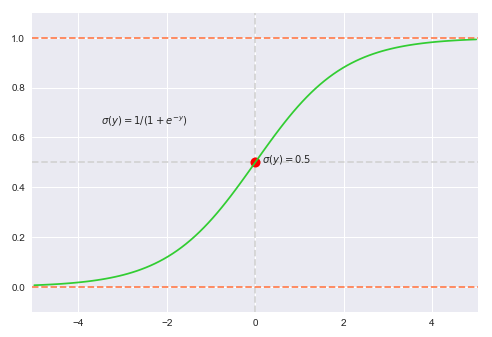
The equation $\color{blue} (A)$ from above is the mathematical model for Logistic Regression. The above function for $p(X)$ is called as a Sigmoid (or Logit) function.

The following illustration displays the plot of a sigmoid function from the equation $\color{blue} (A)$ shown above:

By applying a threshold to the sigmoid function, such as $p(X) \ge 0.5$ to predict class $1$, one can leverage it for binary classification.

Realize the equation $\color{blue}(A)$ from above is non-linear in nature, meaning, we cannot relate how a unit increase in $\beta$ will effect the predicted target value.

We can gain some insights from the sign of the $\beta$ coefficients, which are as follows:

• Positive Coefficient - Increase in the likelihood of the predicted target value belonging to class $1$ (or success)

• Negative Coefficient - Decrease in the likelihood of the predicted target value belonging to class $1$ (or success)

As for the magnitude of the $\beta$ coefficients, one can compare one against the other to gain insights as to which of the features have a stronger influence on the predicted target value. For example, a positive $\beta_1$ that is larger in value (magnitude) than $\beta_2$ has more effect on the predicted target value.

To find the optimum values for the $\beta$ coefficients, the optimization goal of Logistic Regression is to find the sigmoid line of best fit. For that, Logistic Regression uses the idea of Maximum Likelihood, which tries to predict the target values as close as possible to $1$ for all the samples that belong to class $1$ (or success) and as close as possible to $0$ for the samples that belong to class $0$ (or failure).

In mathematical terms, the equation for the maximum likelihood estimate (or cost function) can be represented as follows:

    $L(\beta) = \prod_{i=1}^m p(X_i)^{y_i} (1 - p(X_i))^{(1 - y_i)}$ ..... $\color{red} (7)$

where there are $m$ samples and $i$ is index to represent the $i_{th}$ sample.

*** Basic Rules Logarithms ***

  1. $log_e = \ln$

  2. $\ln(1) = 0$

  3. $\ln(a \times b) = \ln(a) + \ln(b)$

  4. $\ln(a \div b) = \ln(a) - \ln(b)$

  5. $\ln(a^b) = b.\ln(a)$

  6. $\ln(e^a) = a$

Applying natural logarithm to both side of the equation $\color{red} (7)$ from above, we get the following:

    $\ln(L(\beta)) = \ln(\prod_{i=1}^m p(X_i)^{y_i} (1 - p(X_i))^{(1 - y_i)})$

Applying the rules $3$ and $5$ of logarithms to the right hand side, we get the following:

    $\ln(L(\beta)) = \sum_{i=1}^m [y_i.\ln(p(X_i)) + (1 - y_i).\ln(1 - p(X_i))]$

Expanding and re-arranging, we get the following:

    $\ln(L(\beta)) = \sum_{i=1}^m [y_i.\ln(p(X_i)) - y_i.\ln(1 - p(X_i)) + \ln(1 - p(X_i))]$

Pulling the common $y_i$ term out, we get the following:

    $\ln(L(\beta)) = \sum_{i=1}^m [y_i.(\ln(p(X_i)) - \ln(1 - p(X_i))) + \ln(1 - p(X_i))]$

Applying the rule $4$ of logarithms to the right hand side, we get the following:

    $\ln(L(\beta)) = \sum_{i=1}^m [y_i.\ln({\Large{\frac{p(X_i)}{1 - p(X_i)}}})$ $+ \ln(1 - p(X_i))]$

Using the equation $\color{red} (6)$ from above, we get the following:

    $\ln(L(\beta)) = \sum_{i=1}^m [y_i.\ln(X_i\beta) + \ln(1 - p(X_i))]$

Applying the rule $6$ of logarithms to the right hand side, we get the following:

    $\ln(L(\beta)) = \sum_{i=1}^m [y_iX_i\beta + \ln(1 - p(X_i))]$

Using the equation $\color{blue} (A)$ from above, we get the following:

$\color{red} \boldsymbol{\ln(L(\beta))}$ $=$ $\bbox[pink,2pt]{\sum_{i=1}^m [y_iX_i\beta - \ln(1 + e^{X_i\beta})]}$ ..... $\color{blue} (B)$

For simplicity, let $l(\beta) = \ln(L(\beta))$.

In order to find the maximum likelihood estimates (or MLE), one needs to take the partial derivative of the equation $\color{blue} (B)$ from above, which results in the following optimization equation:

    $\Large{\frac{\partial{l(\beta)}}{\partial{\beta}}}$ $= \sum_{i=1}^m [$ $y_iX_i - \Large{\frac{ X_ie^{X_i\beta}}{1 + e^{X_i\beta}}}$ $]$

Rearranging and simplifying, we get the following:

$\color{red} \boldsymbol{\Large{\frac{\partial{l(\beta)}}{\partial{\beta}}}}$ $=$ $\bbox[pink,2pt]{\sum_{i=1}^m X_i[y_i - p(X_i)]}$ ..... $\color{blue} (C)$

In order to find an approximation for the $\beta$ coefficients, one needs to solve the equation $\color{blue} (C)$ from above using numerical methods (such as gradient descent).

Model Evaluation Metrics

In the following paragraphs we will look at the different metrics that help us evaluate the effectiveness of the logistic regression model.

Confusion Matrix

Confusion Matrix (or Error Matrix) is a summary matrix that can be used to evaluate the performance of a classification model.

The following illustration shows the confusion matrix for the logistic regression (binary classification) model:

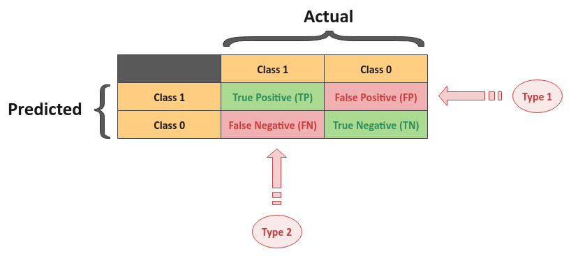
In the confusion matrix above, class $1$ means success or positive, while class $0$ means failure or negative. Also, the columns (top) represents the actual classification, while the rows (left) represents the predicted classification.

The following are the four possible outcomes:

• True Positive - TP for short, it indicates the predicted value of $1$ and the actual value is also $1$

• False Positive - FP for short, it indicates the predicted value of $1$, while the actual value is $0$. This is also known as the Type 1 error

• False Negative - FN for short, it indicates the predicted value of $0$, while the actual value is $1$. This is also known as the Type 2 error

• True Negative - TN for short, it indicates the predicted value of $0$ and the actual value is also $0$

Accuracy

Accuracy is a metric that represents the number of correctly classified data samples over the total number of data samples.

In mathematical terms,

$\color{red} \boldsymbol{Accuracy}$ $= \bbox[pink,2pt]{\Large{\frac{TP + TN}{TP + FP + FN + TN}}}$

Precision

Precision is a metric that represents the number of correctly classified class $1$ (positive) data samples over the total number of actual classified data samples.

In mathematical terms,

$\color{red} \boldsymbol{Precision}$ $= \bbox[pink,2pt]{\Large{\frac{TP}{TP + FP}}}$

Recall

Recall (also known as Sensitivity) is a metric that represents the number of correctly classified class $1$ (positive) data samples over the total number of actual class $1$ (positive) data samples.

In mathematical terms,

$\color{red} \boldsymbol{Recall}$ $= \bbox[pink,2pt]{\Large{\frac{TP}{TP + FN}}}$

F1 - Score

F1 - Score is a metric that represents the weighted average of precision and recall.

In mathematical terms,

$\color{red} \boldsymbol{F1-Score}$ $= \bbox[pink,2pt]{2 \times \Large{\frac{Precision \times Recall}{Precision + Recall}}}$

Receiver Operating Characteristics Curve

The Receiver Operating Characteristics (also known as the ROC) curve is used to visualize the performance of a classification model (such as the logistic regression model) for all possible classification thresholds.

The plot uses the following two terms:

• True Positive Rate - TPR for short. When the actual classification is a $1$, how often did the model correctly predict a $1$. In mathematical terms, it is defined as: $TPR = \Large{\frac{TP}{TP + FN}}$

• False Positive Rate - FPR for short. When the actual classification is a $0$, how often did the model incorrectly predict a $1$. In mathematical terms, it is defined as: $FPR = \Large{\frac{FP}{FP + TN}}$

ROC curve is a plot of the False Positive Rate (FPR) along the x-axis versus the True Positive Rate (TPR) along the y-axis for the different classification thresholds.

The following illustration shows a hypothetical ROC curve:

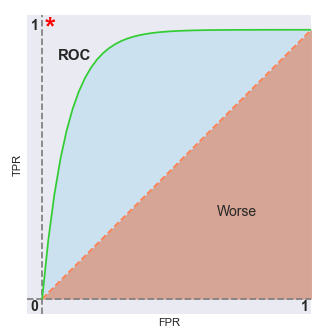
The red dotted line that divides the graph into two halfs is where $TPR = FPR$. Any value on or below this red dotted line is BAD (worse case). The desire is for the ROC curve to be as close as possible to the red star at the top left corner - this is when the classification model is predicting correctly all the time (ideal case).

As we increase the classification threshold, we predict more $0$ values. This implies a lower TPR and FPR. Similarly, as we decrease the classification threshold, we predict more $1$ values. This implies a higher TPR and FPR.

References

Introduction to Probability

© PolarSPARC