Machine Learning - Naive Bayes using Scikit-Learn

Bhaskar S

06/11/2022

Overview

Naive Bayes is a probabilistic classification model, that is based on Bayes Theorem. It is fast, explainable, and good for handling high-dimensional data set. It is called Naive since it makes the simple assumption that all the features in the data set are independent of each other, which is typically not the case in the real world scenarios.

Naive Bayes

In the following sections, we will develop a mathematical intuition for Naive Bayes.

From the article on Bayes Theorem, we can express the relationship between the dependent target variable $y$ and the independent feature variables $x_1, x_2, ..., x_n$ as follows:

$P(y \mid x_1, x_2, ..., x_n) = \Large{\frac{P(x_1, x_2, ..., x_n \mid y) . P(y)}{P(x_1, x_2, ..., x_n)}}$ ..... $\color{red} (1)$

Using the chain rule for conditional probability, we know the following:

$P(a,b,c) = P(a \mid b,c) . P(b,c) = P(a \mid b,c) . P(b \mid c) . P(c)$

Therefore,

$P(x_1, x_2, ..., x_n \mid y) = P(x_1 \mid x_2, ..., x_n \mid y) . P(x_2 \mid x_3, ..., x_n \mid y) ... P(x_n \mid y)$

We know from Naive Bayes that each feature variable $x_i$ is independent of the other.

Therefore,

$P(x_1, x_2, ..., x_n \mid y) = P(x_1 \mid y) . P(x_2 \mid y) ... P(x_n \mid y)$ ..... $\color{red} (2)$

Also,

$P(x_1, x_2, ..., x_n) = P(x_1) . P(x_2) ... P(x_n)$ ..... $\color{red} (3)$

Substituting equations $\color{red} (2)$ and $\color{red} (3)$ into equation $\color{red} (1)$, we get:

$P(y \mid x_1, x_2, ..., x_n) = \Large{\frac{P(x_1 \mid y) . P(x_2 \mid y) ... P(x_n \mid y) . P(y)} {P(x_1) . P(x_2) ... P(x_n)}}$ ..... $\color{red} (4)$

For all samples in the data set, the value of equation $\color{red} (3)$ will be a constant.

Therefore, left-hand side of the equation $\color{red} (4)$ will be proportional to the right-hand side of the equation $\color{red} (4)$ and can be rewriten as follows:

$P(y \mid x_1, x_2, ..., x_n) \propto P(y) . P(x_1 \mid y) . P(x_2 \mid y) ... P(x_n \mid y)$

That is,

$P(y \mid x_1, x_2, ..., x_n) \propto \bbox[pink,2pt]{P(y) . \prod_{i=1}^n P(x_i \mid y)}$ ..... $\color{red} (5)$

The goal of Naive Bayes is then to classify the target variable $y$ into the appropriate category (or class) by finding the maximum likelihood (the right-side of the equation $\color{red} (5)$) that the given set of feature variables $x_1, x_2, ..., x_n$ belong to the appropriate category (or class).

The following are some of the commonly used Naive Bayes algorithms:

Bernoulli Naive Bayes - Used when all the feature variables $x_1, x_2, ..., x_n$ in the data set can only take BINARY values (two values encoded as either a 0 or a 1)
Gaussian Naive Bayes - Used when all the feature variables $x_1, x_2, ..., x_n$ in the data set are CONTINUOUS values that are normally distributed
Multinomial Naive Bayes - Used when all the feature variables $x_1, x_2, ..., x_n$ in the data set are DISCRETE values (like counts or frequencies)

In this following sections, we will demonstrate the use of the Naive Bayes model for classification (using scikit-learn) by leveraging the Glass Identification data set.

The first step is to import all the necessary Python modules such as, pandas, matplotlib, seaborn, and scikit-learn as shown below:

import pandas as pd
import matplotlib.pyplot as plt
import seaborn as sns
from sklearn.preprocessing import StandardScaler
from sklearn.model_selection import train_test_split, GridSearchCV
from sklearn.naive_bayes import GaussianNB
from sklearn.metrics import accuracy_score

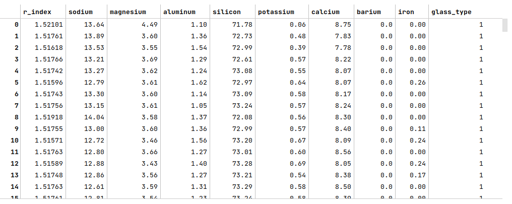
The next step is to load the glass identification data set into a pandas dataframe, set the column names, and then display the dataframe as shown below:

url = 'https://archive.ics.uci.edu/ml/machine-learning-databases/glass/glass.data'
glass_df = pd.read_csv(url, header=None)
glass_df = glass_df.drop(glass_df.columns[0], axis=1)
glass_df.columns = ['r_index', 'sodium', 'magnesium', 'aluminum', 'silicon', 'potassium', 'calcium', 'barium', 'iron', 'glass_type']
glass_df

The following illustration displays few rows from the glass identification dataframe:

Figure.1

The next step is to display information about the glass identification dataframe, such as index and column types, missing (null) values, memory usage, etc., as shown below:

glass_df.info()

The following illustration displays information about the glass identification dataframe:

Figure.2

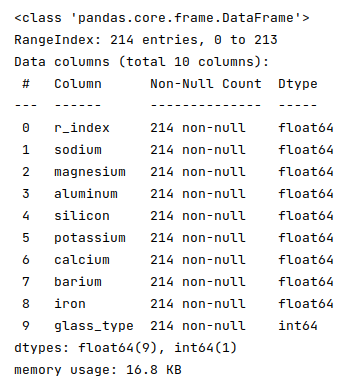
Fortunately, the data seems clean with no missing values.

The next step is to split the glass identification dataframe into two parts - a training data set and a test data set. The training data set is used to train the classification model and the test data set is used to evaluate the classification model. In this use case, we split 75% of the samples into the training dataset and remaining 25% into the test dataset as shown below:

X_train, X_test, y_train, y_test = train_test_split(glass_df, glass_df['glass_type'], test_size=0.25, random_state=101)
X_train = X_train.drop('glass_type', axis=1)
X_test = X_test.drop('glass_type', axis=1)

The next step is to create an instance of the standardization scaler to scale the desired feature (or predictor) variables in both the training and test dataset as shown below:

scaler = StandardScaler()
s_X_train = pd.DataFrame(scaler.fit_transform(X_train), columns=X_train.columns, index=X_train.index)
s_X_test = pd.DataFrame(scaler.fit_transform(X_test), columns=X_test.columns, index=X_test.index)

The next few steps is to visualize the distribution of the feature variables to determine the type of Naive Bayes algorithm to use.

The next step is to display a distribution plot for the feature r_index (refractive index) using the glass identification training data set as shown below:

sns.displot(X_train, x='r_index', color='salmon', kind='kde')
plt.show()

The following illustration shows the distribution plot for the feature r_index from the glass identification training data set:

$Refractive Index$

Figure.3

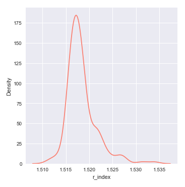
From the distribution plot above, we can infer that the feature r_index seems to be normally distributed.

The next step is to display a distribution plot for the feature aluminum using the glass identification training data set as shown below:

sns.displot(X_train, x='aluminum', color='limegreen', kind='kde')
plt.show()

The following illustration shows the distribution plot for the feature aluminum from the glass identification training data set:

Figure.4

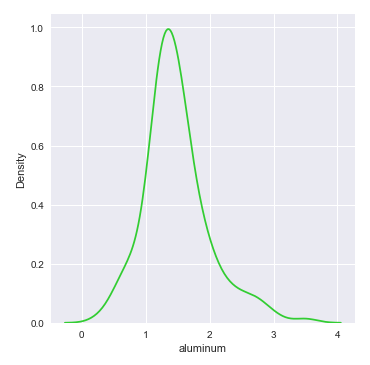
From the distribution plot above, we can infer that the feature aluminum seems to be normally distributed.

The next step is to display a distribution plot for the feature barium using the glass identification training data set as shown below:

sns.displot(X_train, x='barium', color='dodgerblue', kind='kde')
plt.show()

The following illustration shows the distribution plot for the feature barium from the glass identification training data set:

Figure.5

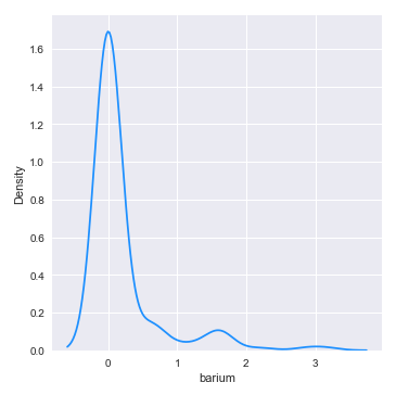
From the distribution plot above, we can infer that the feature barium seems almost normally distributed.

The next step is to display the distribution plot (along with the scatter plot) for the remaining features using the glass identification training data set as shown below

sns.pairplot(glass_df[['calcium', 'iron', 'magnesium', 'silicon', 'sodium']], height=1.5, diag_kind='kde')
plt.show()

The following illustration shows the distribution plot (along with the scatter plot) for the remaining features using the glass identification training data:

Figure.6

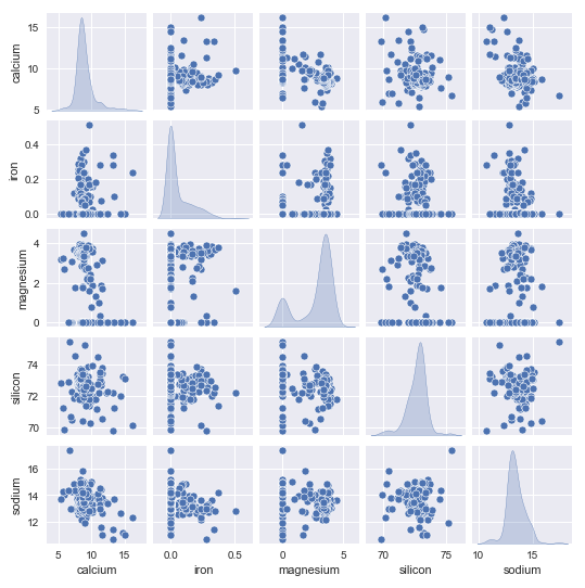
From the pair plot above, we can infer that the remaining features seems normally distributed.

Given that all the feature variables from the glass identification data set seem normally distributed, the next step is to initialize the Gaussian Naive Bayes model class from scikit-learn and train the model using the training data set as shown below:

model = GaussianNB()
model.fit(s_X_train, y_train)

The next step is to use the trained model to predict the glass_type using the test dataset as shown below:

y_predict = model.predict(s_X_test)

The next step is to display the accuracy score for the model performance as shown below:

accuracy_score(y_test, y_predict)

The following illustration displays the accuracy score for the model performance:

Figure.7

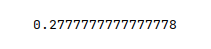
From the above, one can infer that the model seems to predict very poorly. One possible reason could be that the model is not using an optimal hyperparameter value.

One of the hyperparameters used by the Gaussian Naive Bayes is var_smoothing, which controls the variance of all the feature variables such that the distribution curve could be widen to include more samples away from the mean.

The next step is to perform an extensive grid search on a list of hyperparameter values to determine the optimal value of the hyperparameter var_smoothing and display the optimal value as shown below:

parameters = {
  'var_smoothing': [1e-2, 1e-3, 1e-4, 1e-5, 1e-6, 1e-7, 1e-8, 1e-9, 1e-10, 1e-11, 1e-12, 1e-13, 1e-14, 1e-15]
}
cv_model = GridSearchCV(estimator=model, param_grid=parameters, cv=5, verbose=1, scoring='accuracy')
cv_model.fit(s_X_train, y_train)
cv_model.best_params_

The following illustration displays the optimal value for the hyperparameter var_smoothing:

Figure.8

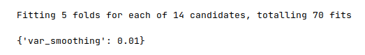
The next step is to re-initialize the Gaussian Naive Bayes model with the hyperparameter var_smoothing set to the value of 0.01 and re-train the model using the training data set as shown below:

model = GaussianNB(var_smoothing=0.01)
model.fit(s_X_train, y_train)

The next step is to use the trained model to predict the glass_type using the test dataset as shown below:

y_predict = model.predict(s_X_test)

The final step is to display the accuracy score for the model performance as shown below:

accuracy_score(y_test, y_predict)

The following illustration displays the accuracy score for the model performance:

Figure.9

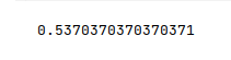
From the above, one can infer that the model seems to predict much better now (not great).

Hands-on Demo

The following is the link to the Jupyter Notebook that provides an hands-on demo for this article:

Naive Bayes

References

Introduction to Probability

Introduction to Bayes Theorem