Figure.1
| PolarSPARC |
Machine Learning - Decision Trees using Scikit-Learn
| Bhaskar S | 06/24/2022 |
Decision Trees
Whether we realize it or not, we are constantly making decisions to arrive at desired outcomes. When presented with a lot of options, we iteratively ask question(s) to narrow the options till we arrive at the desired outcome. This process forms a tree like structure called a Decision Tree.
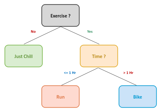
The following is an illustration of a very simple decision tree:
The following are some terminology related to decision trees:
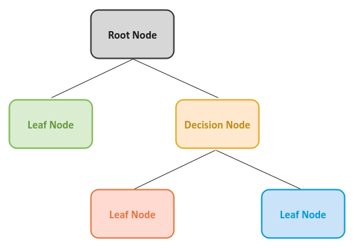
Root Node :: the node at the top of the decision tree
Decision Node :: the sub-node or child node of the decision tree where a decision is made or a condition is evaluated
Splitting :: the process of dividing the data at a decision node further into two children nodes, based on a condition being true or false
Leaf Node :: the terminal node of the decision tree, which cannot be split further, and represents a specific class (or category)
Depth :: the longest path from the root node to a leaf node
The following is an illustration of a decision tree with the various node types:
In short, a Decision Tree is a machine learning algorithm, in which data is classified by iteratively splitting the data, based on some condition(s) on the feature variable(s) from the data set.
The Decision Tree machine learning algorithm can be used for either classification or regression problems. Hence, a Decision Tree is often referred to by another name called Classification and Regression Tree (or CART for short).
However, in reality, Decision Trees are more often used for solving classification problems.
Now, the question one may ask - how does the Decision Tree algorithm choose a feature variable and make the determination to split the node ??? This is where the Gini Impurity comes into play.
Gini Impurity is mathematically defined as follows:
$G = \sum_{c=1}^N p_c(1 - p_c) = p_1(1 - p_1) + p_2(1 - p_2) + \ldots + p_N(1 - p_N) = (p_1 + p_2 + \ldots + p_N) - \sum_{c=1}^N p_c^2 = 1 - \sum_{c=1}^N p_c^2$
where $N$ is the number of classes (or categories), $p_c$ is the probability of a sample with class (or category) $c$ being chosen, and $1 - p_c$ is the probability of mis-classifying a sample.
Note that $p_1 + p_2 + \ldots + p_N = 1$
In the following sections, we will develop an intuition for Gini Impurity using a simple case of binary classification (two classes or categories or labels) - a red diamond and a blue square.
The following illustration depicts the combination of five classified samples in a node:
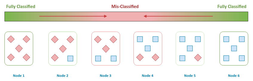
For either Node 1 OR Node 6, all the samples have been classified into one of the two categories and are considered 100% correctly classified.
Next, in the spectrum, for either Node 2 OR Node 5, all except one of the samples have been correctly classified into one of the two categories and are considered 80% classified. The remaining 20% are mis-classified.
Finally, for either Node 3 OR Node 4, all except two of the samples have been correctly classified into one of the two categories and are considered 60% classified. And, the remaining 40% are mis-classified.
Given the above facts, the idea of Gini Impurity is then to minimize the impurity (mis-classification) at each node during the data splits.
The following illustration depicts the combination of five classified samples in a node, along with their Gini Impurity (at the bottom):
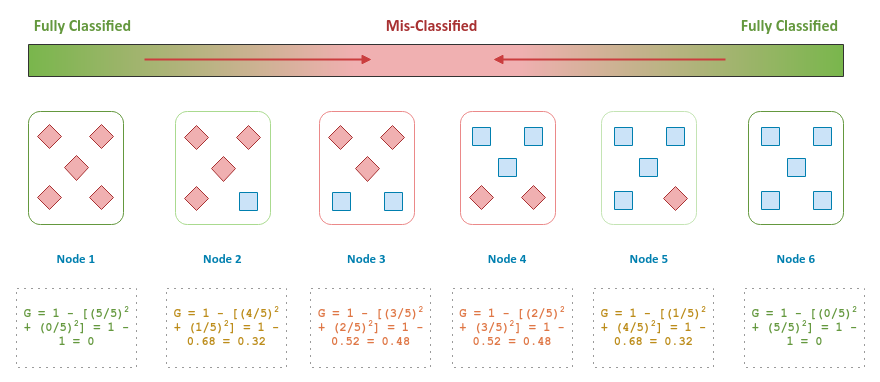
Notice that the Gini Impurity has a perfect score of 0 (zero), when all the samples in a node are correctly classified (Node 1 OR Node 6).
In other words, the decision tree algorithm performs the data split at a node with the goal of minimizing the Gini Impurity score. The algorithm performs the splits iteratively till the Gini Impurity score is zero, at which point the target is classified into one of the categories.
Similarly, to choose the feature variable for the root node, the decision tree algorithm computes the Gini Impurity score for all the feature variables and picks the feature variable with the lowest Gini Impurity value.
The following are some of the advantages of decision trees:
Easy to explain, interpret, and visualize
Can handle any type of data - be it categorical or numerical
No need to perform data normalization or scaling
Will automatically pick features that are important
The following are some of the disadvantages of decision trees:
Can easily overfit if not controlled
Changes in the training data impact the structure of the tree, resulting in instability
In this following sections, we will demonstrate the use of the Decision Tree model for classification (using scikit-learn) by leveraging the same Glass Identification data set we have been using until now.
The first step is to import all the necessary Python modules such as, pandas, matplotlib, seaborn, and scikit-learn as shown below:
import pandas as pd
import matplotlib.pyplot as plt
import seaborn as sns
from sklearn.model_selection import train_test_split
from sklearn.tree import DecisionTreeClassifier, plot_tree
from sklearn.metrics import accuracy_score
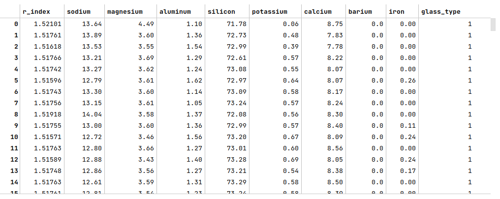
The next step is to load the glass identification data set into a pandas dataframe, set the column names, and then display the dataframe as shown below:
url = 'https://archive.ics.uci.edu/ml/machine-learning-databases/glass/glass.data'
glass_df = pd.read_csv(url, header=None)
glass_df = glass_df.drop(glass_df.columns[0], axis=1)
glass_df.columns = ['r_index', 'sodium', 'magnesium', 'aluminum', 'silicon', 'potassium', 'calcium', 'barium', 'iron', 'glass_type']
glass_df
The following illustration displays few rows from the glass identification dataframe:
The next step is to display information about the glass identification dataframe, such as index and column types, missing (null) values, memory usage, etc., as shown below:
glass_df.info()
The following illustration displays information about the glass identification dataframe:
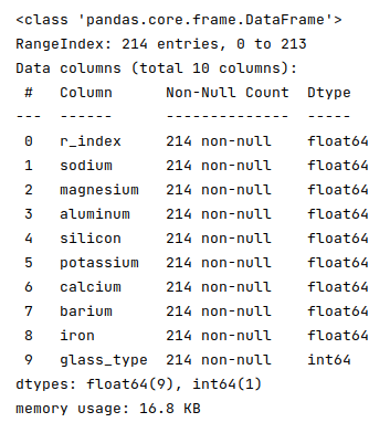
Fortunately, the data seems clean with no missing values.
The next step is to display the count of each of the target classes (or categories) in the glass identification dataframe as shown below:
glass_df['glass_type'].value_counts()
The following illustration displays the count of each of the target classes from the glass identification dataframe:
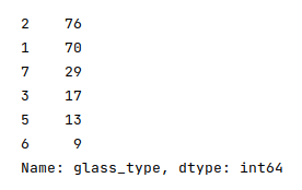
Notice that there are values for SIX (6) types of glasses.
The next step is to split the glass identification dataframe into two parts - a training data set and a test data set. The training data set is used to train the classification model and the test data set is used to evaluate the classification model. In this use case, we split 75% of the samples into the training dataset and remaining 25% into the test dataset as shown below:
X_train, X_test, y_train, y_test = train_test_split(glass_df, glass_df['glass_type'], test_size=0.25, random_state=101)
With Decision Trees, one does *NOT* have to scale the feature (or predictor) variables.
The next step is to display the correlation matrix of the feature (or predictor) variables with the target variable as shown below:
sns.heatmap(X_train.corr(), annot=True, cmap='coolwarm', fmt='0.2f', linewidth=0.5)
plt.show()
The following illustration displays the correlation matrix of the feature from the glass identification dataframe:
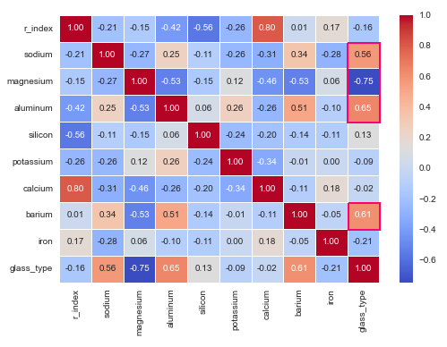
From the correlation matrix above, notice that some of the features (annotated in red) have a strong relation with the target variable.
The next step is to drop the target variable from the training and test dataset as shown below:
X_train = X_train.drop('glass_type', axis=1)
X_test = X_test.drop('glass_type', axis=1)
The next step is to initialize the Decision Tree model class from scikit-learn and train the model using the training data set as shown below:
model1 = DecisionTreeClassifier(random_state=101)
model1.fit(X_train, y_train)
The next step is to use the trained model to predict the glass_type using the test dataset as shown below:
y_predict = model1.predict(X_test)
The next step is to display the accuracy score for the model performance as shown below:
accuracy_score(y_test, y_predict)
The following illustration displays the accuracy score for the model performance:

From the above, one can infer that the model seems to predict okay.
The following illustration depicts the visual representation of the decision tree:
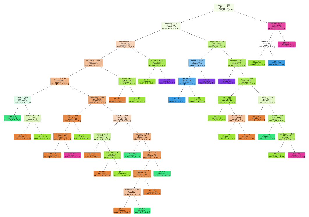
One of the challenges with a Decision Tree model is that it can overfit using the training model to create a deeply nested (large depth) tree.
One of the hyperparameters used by the Decision Tree classifier is max_depth, which controls the maximum depth of the tree.
The next step is to re-initialize the Decision Tree class with the hyperparameter max_depth set to the value of 5 and re-train the model using the training data set as shown below:
model2 = DecisionTreeClassifier(max_depth=5, random_state=101)
model2.fit(X_train, y_train)
The next step is to use the re-trained model to predict the glass_type using the test dataset as shown below:
y_predict = model2.predict(X_test)
The next step is to display the accuracy score for the model performance as shown below:
accuracy_score(y_test, y_predict)
The following illustration displays the accuracy score for the model performance:
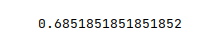
From the above, one can infer that the model seems to predict much better now.
The following illustration depicts the visual representation of the improved decision tree:
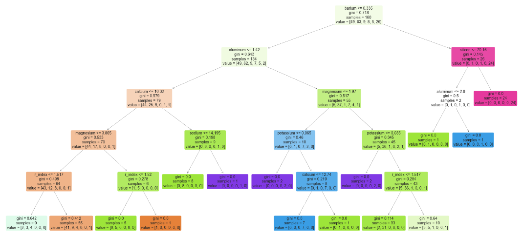
Let us look at the following simpler visual representation of the decision tree to explain how to interpret the contents of a node in the decision tree:
Feature Criteria :: represents the decision criteria using a feature variable. In this example, the node is testing for barium &le 0.335
Gini Impurity Score :: represents the gini impurity value at the node. In this example, the node has a gini impurity score of 0.718
Sample Size :: represents the size of the sample (number of rows from the training data set). In this example, the node is dealing with a sample size of 160
Class Distribution :: represents how many samples fall into the different classes (or categories). In this example, the node has classified 49 samples into class 1, 63 samples into class 2, and so on
IMPORTANT - One may be wondering what was the purpose of the correlation heatmap above (Figure.8). While the feature silicon may have had a poor correlation with the target glass_type, take look at the decision tree(s) from above (Figure.12 or Figure.13) - the feature silicon seems to have an influence on the target classification.
Hands-on Demo
The following is the link to the Jupyter Notebook that provides an hands-on demo for this article: