Figure.1
| PolarSPARC |
Machine Learning - Understanding Cross Validation
| Bhaskar S | 06/03/2022 |
Overview
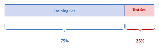
Until now in this series, the approach taken to build and evaluate a machine learning model was to split the given data set into two sets - a training set and a test set. The training set typically comprises of about 70% to 80% of the data from the original data set.
The following illustration depicts this train-test split:
The question - why do we take this approach ??? The hypothesis is that, we train the model on one data set and evaluate the model using a different data set that the model has never seen before, with the belief that the result from the test data set would mimic the behavior of the model with an unseen data in the future.
Cross Validation is the process of evaluating the accuracy of any machine learning model with new unseen data, so that the model is generalized enough for future predictions.
The simple cross validation approach of splitting a given data set into a training set and a test set that we have been using until now is often referred to as the Hold Out cross validation method.
A typical machine learning pipeline is to build a generalized model (for the given problem space) that can predict with a reasonably high accurately on the future data points. The pipeline involves the following steps:
Train-test split
Fit model using train set
Evaluate model using test set
Measure model accuracy
Select new model if accuracy low
Go to Step 2
The following illustration depicts this machine learning pipeline:
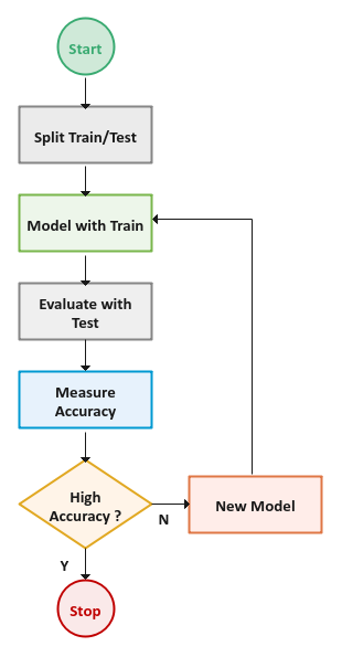
Note that the selection of the new model could be either adjusting the hyperparameters or choosing a different algorithm.
However, there is an issue with the pipeline described above - we do *NOT* have any separate truly unseen data (that is different from the test set) to evaluate the final model selected from the pipeline.
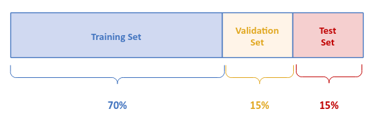
An enhancement to the simple cross validation hold out method is to split the given data set into three sets - a training set, a validation set, and a test set. The training set typically comprises of about 70% of the data from the original data set and the validation set typically comprises of about 15% of the remaining data.
The following illustration depicts this train-validate-test split:
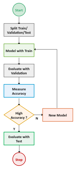
The following illustration depicts the enhanced machine learning pipeline:
One of the challenges with the Hold Out cross validation method is that the model accuracy measure from the test set may have high variance depending on what samples end up in the test set. In other words, the model accuracy measure depends on what data samples end up in the test set.
In order to address the variation challenges from the uneven distribution of the data samples in the test set, the k-Fold cross validation method is used.
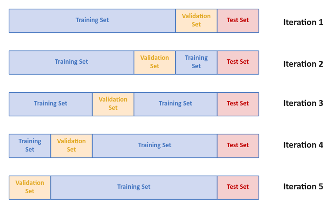
In the k-Fold cross validation method, the given data set is first split into the training and test sets. Then, the training set is split into into $k$ parts (or folds) of equal size. The value of $k$ is typically 5 or 10. In each iteration, use the next fold from the $k$ folds as the validation set and the combination of the remaining $k-1$ folds as the training set.
For $k = 5$, the following illustration depicts the k-fold cross validation:
The pipeline with the k-fold cross validation involves the following steps:
Perform a Train-test split
Split the training set into $k$ folds
Select the next fold from $k$ folds as the validation set
New training set is the combination remaining $k-1$ folds
Fit model using the new training set
Evaluate the model using the validation set
Measure the model accuracy and save the result
Continue Steps 3 through 7 for $k$ iterations
Compute the average of the $k$ model accuracy scores
Select new model if the average model accuracy is low
Go to Step 3
Finally evaluate selected model using the test set
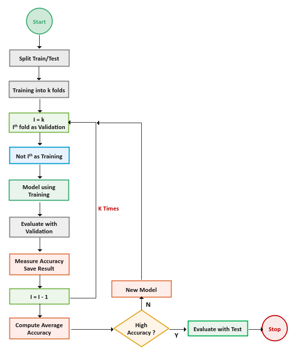
The following illustration depicts the k-fold cross validation machine learning pipeline:
Cross Validation using Scikit-Learn
In this article, we will use the Diamond Prices data set to demonstrate cross validation for selecting model hyperparameter(s).
The first step is to import all the necessary Python modules such as, pandas, and scikit-learn as shown below:
import pandas as pd
from sklearn.preprocessing import StandardScaler
from sklearn.model_selection import train_test_split, KFold, cross_val_score
from sklearn.linear_model import Ridge
from sklearn.metrics import r2_score
The next step is to load and display the Diamond Prices dataset into a pandas dataframe as shown below:
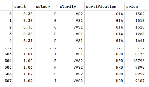
url = './data/diamond-prices.csv'
diamond_prices_df = pd.read_csv(url, usecols=['carat', 'colour', 'clarity', 'certification', 'price'])
diamond_prices_df
The following illustration shows the few rows of the diamond prices dataframe:
The next step is to display the count for all the missing values from the diamond prices dataframe as shown below:
diamond_prices_df.isnull().sum()
The following illustration shows the count for all the missing values from the diamond prices dataframe:
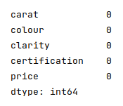
This is to ensure we have no missing values in the diamond prices data set.
The next step is to identify all the ordinal features from the diamond prices and creating a Python dictionary whose keys are the names of the ordinal features and their values are a Python dictionary of the mapping between the labels (of the ordinal feature) to the corresponding numerical values as shown below:
ord_features_dict = {
  'colour': {'D': 6, 'E': 5, 'F': 4, 'G': 3, 'H': 2 , 'I': 1},
  'clarity': {'IF': 5, 'VVS1': 4, 'VVS2': 3, 'VS1': 2, 'VS2': 1}
}
The next step is to map the categorical labels for each of the ordinal features from the diamond prices dataframe into their their numerical representation using the Python dictionary from above as shown below:
for key, val in ord_features_dict.items():
  diamond_prices_df[key] = diamond_prices_df[key].map(val)
diamond_prices_df
The following illustration shows the few rows of the transformed diamond prices dataframe:
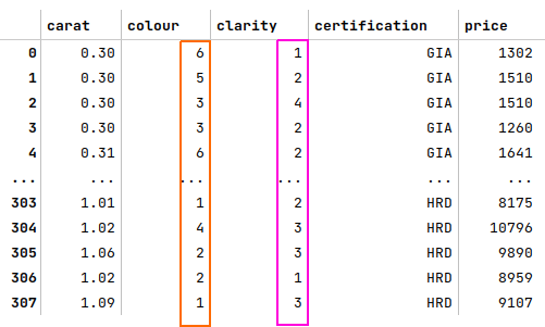
Notice the annotated columns with transformed ordinal feature values - they are all numerical now.
The next step is to create dummy binary variables for the nominal feature 'certification' from the diamond prices data set as shown below:
cert_encoded_df = pd.get_dummies(diamond_prices_df[['certification']], prefix_sep='.', sparse=False)
cert_encoded_df
The following illustration displays the dataframe of all dummy binary variables for the nominal feature 'certification' from the diamond prices dataframe:
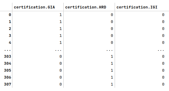
Notice that, with the dummy binary variables generation, we have created 3 additional features above.
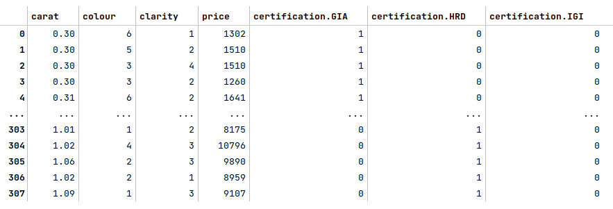
The next step is to drop the nominal feature from the diamond prices dataframe, merge the dataframe of dummy binary variables we created earlier, and display the merged diamond prices dataframe as shown below:
diamond_prices_df = diamond_prices_df.drop('certification', axis=1)
diamond_prices_df = pd.concat([diamond_prices_df, cert_encoded_df], axis=1)
diamond_prices_df
The following illustration displays few rows from the merged diamond prices dataframe:
The next step is to first split the diamond prices dataframe into two parts - a other data set and a test data set. Then, we split the other data set into the training data set (used to train the regression model) and the validation data set used to evaluate the regression model as shown below:
X_other, X_test, y_other, y_test = train_test_split(diamond_prices_df[['carat', 'colour', 'clarity', 'certification.GIA', 'certification.HRD', 'certification.IGI']], diamond_prices_df['price'], test_size=0.15, random_state=101)
X_train, X_val, y_train, y_val = train_test_split(X_other, y_other, test_size=0.15, random_state=101)
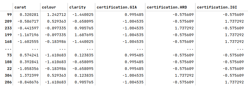
The next step is to create an instance of the standardization scaler to scale all the feature variables from the other, training, validation, and test data set as shown below:
scaler = StandardScaler()
X_other_s = pd.DataFrame(scaler.fit_transform(X_other), columns=X_other.columns, index=X_other.index)
X_train_s = pd.DataFrame(scaler.fit_transform(X_train), columns=X_train.columns, index=X_train.index)
X_val_s = pd.DataFrame(scaler.transform(X_val), columns=X_val.columns, index=X_val.index)
X_test_s = pd.DataFrame(scaler.transform(X_test), columns=X_test.columns, index=X_test.index)
X_train_s
The following illustration displays few rows from the scaled diamond prices dataframe:
In the following sections, we will demonstrate the two cross validation approaches - the Hold Out Train-Validate-Test method and the k-Fold method, using the regularized Ridge regression model.
Hold Out Train-Validate-Test
The next step is to perform the Ridge regression with the hyperparamter 'alpha' set to $100$. We fit the model using the training data set, evaluate the model using the validation data set, and display the $R2$ score as shown below:
model_one = Ridge(alpha=100)
model_one.fit(X_train_s, y_train)
y_val_pred1 = model_one.predict(X_val_s)
r2_score(y_val, y_val_pred1)
The following illustration displays the $R2$ score for the Ridge regression with the hyperparamter 'alpha' set to $100$:
The next step is to perform the next iteration of the Ridge regression with the hyperparamter 'alpha' set to $5$. Again, we fit the model using the training data set, evaluate the model using the validation data set, and display the $R2$ score as shown below:
model_two = Ridge(alpha=5)
model_two.fit(X_train_s, y_train)
y_val_pred2 = model_two.predict(X_val_s)
r2_score(y_val, y_val_pred2)
The following illustration displays the $R2$ score for the Ridge regression with the hyperparamter 'alpha' set to $5$:
Given the $R2$ score for the second model is better, the next step is to perform a final model evaluation using the test data set and display the $R2$ score as shown below:
y_pred = model_two.predict(X_test_s)
r2_score(y_test, y_pred)
The following illustration displays the $R2$ score from the final model evaluation using the test data set:
k-Fold
The next step is to create an instance of KFold with $5$ folds as shown below:
folds_5 = KFold(n_splits=5, random_state=101, shuffle=True)
The next step is to perform a 5-fold cross validation on the Ridge regression model with the hyperparamter 'alpha' set to $100$. One needs to specify an instance of the model, the other data set, and the scoring method ($R2$ in our case) to the function cross_val_score, which under-the-hood performs the necessary 5-fold cross validation. On completion, it returns an array of $R2$ scores (one for each of the 5 iterations). We then perform an average on the scores as shown below:
model_one = Ridge(alpha=100)
scores = cross_val_score(model_one, X_other_s, y_other, scoring='r2', cv=folds_5)
scores.mean()
The following illustration displays the average $R2$ score for the Ridge regression with the hyperparamter 'alpha' set to $100$:
The next step is to perform another iteration of the 5-fold cross validation on the Ridge regression model with the hyperparamter 'alpha' set to $5$. Once again, we specify the model, the other data set, and the scoring method ($R2$ in our case) to the cross_val_score function, which returns an array of $R2$ scores. We then perform an average on the scores as shown below:
model_two = Ridge(alpha=5)
scores2 = cross_val_score(model_two, X_other_s, y_other, scoring='r2', cv=folds_5)
scores2.mean()
The following illustration displays the average $R2$ score for the Ridge regression with the hyperparamter 'alpha' set to $5$:
Given the $R2$ score for the second model is better, the next step is to perform a final model evaluation using the test data set and display the $R2$ score as shown below:
model_two.fit(X_other_s, y_other)
y_pred = model_two.predict(X_test_s)
r2_score(y_test, y_pred)
Notice that we have to fit the model using the other data set before using the model to predict.
The following illustration displays the $R2$ score from the final model evaluation using the test data set:
Hands-on Demo
The following is the link to the Jupyter Notebooks that provides an hands-on demo for this article: