Introduction to Deep Learning - Part 1

Introduction

Artificial Intelligence has progressed by leaps and bounds over the past few years and hence a lot of buzz around Deep Learning (aka Deep Neural Networks).

Deep Learning is a subset of Machine Learning, which tries to mimic the way the Neurons are connected and process information in the human brain.

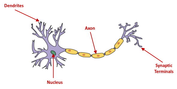
The following illustration depicts the structure of a neuron:

The human brain is a highly interconnected network of about 100 Billion neurons, which have about 100 Trillion connections between them.

A neuron is the basic building block of LEARNING in the human brain and it consists of a single cell called the Nucleus, which is connected to a tree-like nerve extensions referred to as the Dendrites.

Dendrites receives signals from other connected neurons, which in-turn receive signals through the different sensory channels - sight, smell, sound, taste, touch, etc.

The nucleus behaves like a simple processor, acting on the input signal and generating an output signal. The output signal is sent to other connected neurons via the transmission channel referred to as the Axon.

The axon terminates at the Synatic Terminals, which in-turn connect to other neurons.

The synatic terminals act like the memory in the human brain.

In other words, a neuron acts like a simple computational unit and a billion of these connected neurons is what creates the AMAZING human brain.

The idea of deep neural networks is to mimic the neuron network of the human brain.

In the following sections, we will start to put together the components that will lead to a Deep Neural Network - an artificial human brain.

Perceptron

A Perceptron is an artificial equivalent of a neuron. At a very high-level, it consumes multiple inputs and generates a binary (0 or 1) output.

The following illustration depicts the structure of a perceptron:

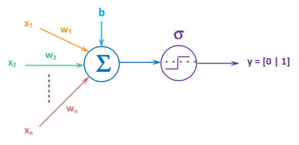
From the illustration in Figure.2 above, we see the perceptron taking inputs perceptron $x_1$ through $x_n$. Each of the inputs $x_i$ have an associated WEIGHT $w_i$. Think of a weight as the importance (or influence) the associated input has on the output. The single adjustment term $b$ is the BIAS, similar to the intercept term in an equation for a line. The term $\Large{\Sigma}$ is the symbol for summation. The output from the summation $\Sigma$ is passed through a function $\sigma$, referred to as the Activation Function, to produce the final output $y$.

In other words, the perceptron takes the sum of weighted inputs along with the bias $b$ and sends it through a transformation function $\sigma$:

    $y = \Large{\sigma}$$(\sum_{i=1}^n w_i.x_i + b)$$..... \color{red}\textbf{(1)}$

    OR, using the matrix notation:

    $y = \Large{\sigma}$$(W.x^T + b)$$..... \color{red}\textbf{(2)}$

to produce the final binary output $y = [0 | 1]$.

If the value of $\sigma(x) \le 0$, the output is $0$ AND if the value of $\sigma(x) \gt 0$, the output is $1$. By default, the activation function $\sigma$ from a perceptron produces a binary value of $0 | 1$. Therefore, the activation function is often referred to as the Step Function (hence a step symbol inside $f$ in the illustration above).

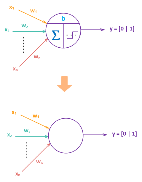
In the illustration Figure.2 above, we show the two functions - the summation $\Sigma$ and the activation function $\sigma$ for clarity. In practice, the bias $b$, the summation operation $\Sigma$ and the activation function $\sigma$ are all represented as a single empty circle as shown in the illustration below:

From the above paragraph(s), one can clearly deduce that a perceptron simply behaves like a Linear Classifier.

To understand the behavior of a single perceptron, let us look at a simple binary classification dataset with two features $X1$ and $X2$. The following illustration depicts the scatter plot of the simple dataset with two classes:

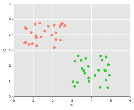
Using a single perceptron with inputs $X1$ and $X2$, one can train the model using the simple dataset and predict the target class on future data values.

After the training, the single perceptron would assume the following values for the two weights $W1$ and $W2$ associated with the input and the bias $b$:

    $W1 = -0.46$

    $W2 = 0.49$

    $b = 0.0$

    The mathematical equation for the perceptron would be: $-0.46.X1 + 0.49.X2$

The following illustration depicts the scatter plot of our simple binary classification dataset, along with the decision boundary of the perceptron that demarcates the two classes:

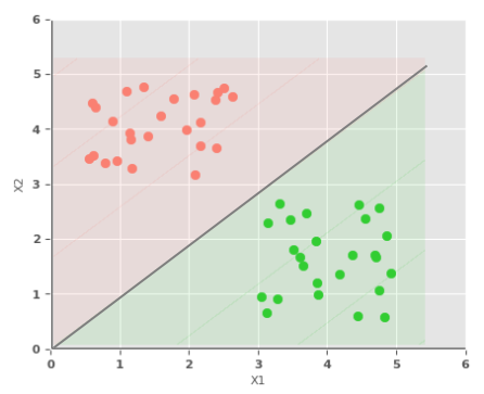
When $X1$ is smaller and $X2$ is larger, the activation function $\sigma$ outputs a $1$, tagging the data as a RED point. Similarly, when $X1$ is larger and $X2$ is smaller, the activation function $\sigma$ outputs a $0$, tagging the data as a GREEN point.

Once again, from the above example, one can confirm that a perceptron behaves like a simple linear classifier.

What if there are more than two inputs to the perceptron ???

From the mathematical equation $\color{red}\textbf{(2)}$ above, it is clear NO MATTER how many inputs a single perceptron takes, it will always behave like a simple linear classifier.

Neural Network

Let us now look at another simple dataset with multple classes using two features $X1$ and $X2$. The following illustration depicts the scatter plot of the multi-class dataset:

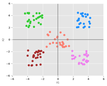
Given that a single perceptron behaves like a simple linear classifier, it would not be able to properly classify the above dataset. This implies we will need multiple perceptrons to handle the above dataset.

As indicated earlier, a perceptron is an artificial equivalent of a neuron in the human brain. We know the human brain is a complex network of neurons. So, how does one create an equvalent network of perceptrons ???

One could connect a series of perceptrons (in layers) starting from the input till the output as shown in the illustration below:

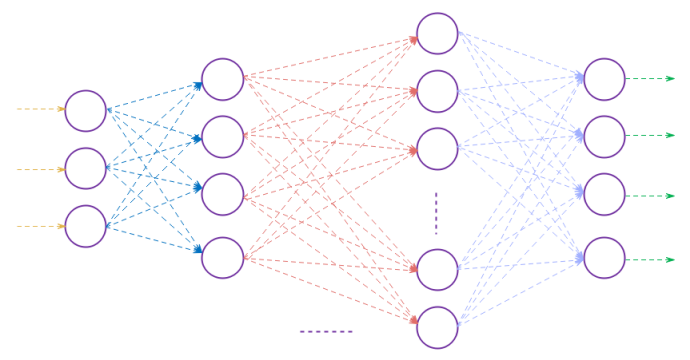
The network of perceptrons depicted in the illustration above is what is referred to as the Deep Neural Network (or simply a Neural Network).

The following illustration shows the core aspects of a Neural Network:

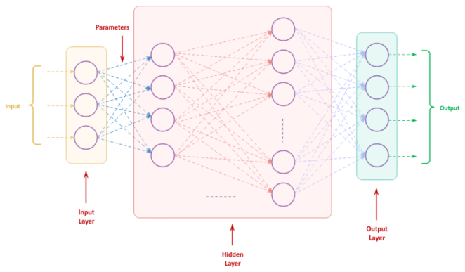
Each column of perceptrons is referred to as a Layer.

The first layer receives the input and is known as the Input Layer. The received input will then pass through a series of one or more layers for further processing, which are referred to as the Hidden Layer(s). The last layer produces the final output and is known as the Output Layer .

Each of the input lines (connections) into a perceptron has an associated weight and each of the perceptrons have an associated bias value. The individual weights and the bias of the perceptron s is often referred to as the Parameters.

To accurately segregate multi-class dataset shown above, we will need a neural network with one hidden layer consisting of five perceptrons as shown in the illustration below:

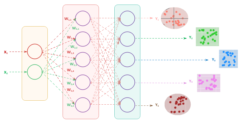
For input $X1$, notice the associated weights from $W_{1,1}$ through $W_{1,5}$ for each of the five perceptrons respectively. Similarly, for input $X2$, the associated weights are from $W_{2,1}$ through $W_{2,5}$.

The following illustration depicts the scatter plot of our simple multi-class dataset, along with the decision boundary as identified by the neural network:

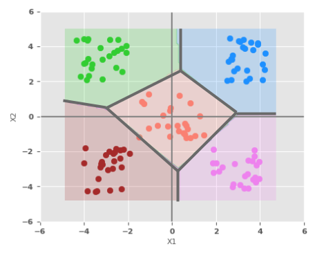
From the decision boundary illustration above, once again we observe the network of perceptrons behave like a simple linear classifier.

Activation Function

In the human brain, based on the situation and context, certain neurons get ACTIVATED and fire signals. Similary, the activation function in a neural network tries to emulate that behavior. As an example, when one encounters a frog walking along a trail, the human brain just focus on the frog, ignoring other things in the surrounding.

The default activation function $\sigma$ associated with a perceptron is a binary step function, which outputs discrete values - a $0$ if $\sigma(x) \le 0$ and a $1$ if $\sigma(x) \gt 0$. This forces the perceptron to behave like a binary classifier.

In other words, a perceptron, by default, would ouput either a $0$ or a $1$. This is like saying lighter shades of grey are same as white and the darker shades of grey are black as shown in the illustration below:

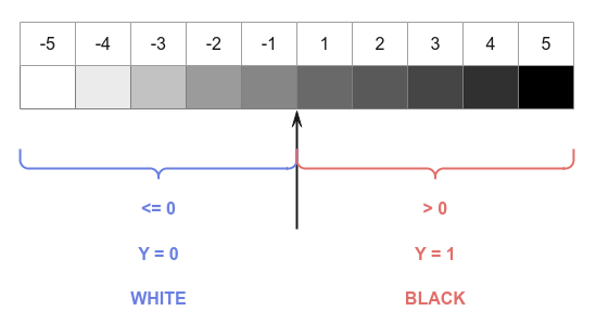
The binary step function works well for linear binary classification use-cases, but many other real-world cases demonstrate a non-linear behavior, which implies continuous values (just like the various shades of grey).

In order to handle many of the real-world use-cases, one can change the default activation function to the other functions as listed below:

• Identify Function :: a linear activation function that produces an output $x$ which is identical to the input $x$.

  In mathematical terms:

      $y = \sigma(x) = x$

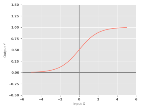
• Sigmoid Function :: a non-linear activation function, also referred to as the Logistic Function, produces an output in the range of $0$ to $1$ for a given input.

  In mathematical terms:

      $y = \sigma(x) = \Large{\frac{1}{1 + e^{-x}}}$

  The following illustration shows the graph of a sigmoid activation function:

  
  
  

  Figure.12
  
  

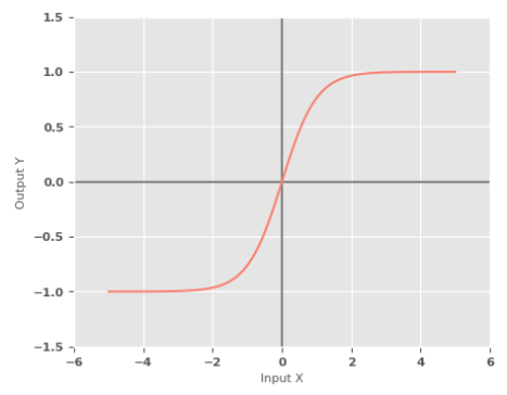
• Tanh Function :: a non-linear activation function, also referred to as the Hyperbolic Tangent Function, produces an output in the range of $-1$ to $1$ for a given input.

  In mathematical terms:

      $y = \sigma(x) = \Large{\frac{e^x - e^{-x}}{e^x + e^{-x}}}$

  The following illustration shows the graph of a tanh activation function:

  
  
  

  Figure.13
  
  

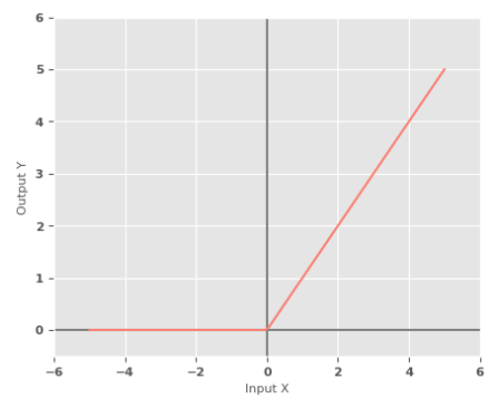
• Rectified Linear Unit Function :: a linear activation function, also referred to as the ReLU Function, produces an output of $max(0, x)$ for a given input x.

  In mathematical terms:

      $y = \sigma(x) = max(0, x)$

  The following illustration shows the graph of a ReLU activation function:

  
  
  

  Figure.14
  
  

© PolarSPARC