Fig.1
Exploring Pandas DataFrame
| Bhaskar S | 01/01/2016 |
Introduction
Pandas is a general purpose Python extension module for performing data manipulation and data analysis. At the core of Pandas is the support for two data structures objects - a one-dimensional DataFrame object and a two-dimensional DataFrame object.
The main features of the Pandas library can be summarized as follows:
Support for a one-dimensional array like structure called a DataFrame
Support for a two-dimensional table like structure called a DataFrame
Built-in support for an index on both DataFrame and DataFrame
Automatic alignment on index during operations for both DataFrame and DataFrame
In this article, we will explore the two-dimensional table like data structure called DataFrame. One can think of a DataFrame to be similar to an Excel spreadsheet or a database table.
Installation and Setup
To make it easy and simple, we choose the open-source Anaconda Python distribution, which includes all the necessary Python packages for science, math, & engineering computations as well as statistical data analysis.
Download the Python 3 version of the Anaconda distribution.
Extract the downloaded archive to a directory, say, /home/abc/anaconda3.
Finally, update the PATH environment variable to include /home/abc/anaconda3/bin.
Hands-on with Pandas DataFrame
Open a terminal window and fire off the IPython Notebook.
To begin using DataFrame, one must import the pandas module as shown below:
import numpy as np
import pandas as pd
Notice we have also imported numpy as we will be using it.
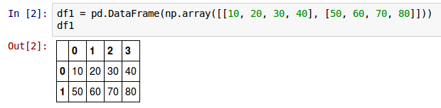
To create a simple 2-rows by 4-columns DataFrame called df1, invoke the DataFrame constructor as shown below:
df1 = pd.DataFrame(np.array([[10, 20, 30, 40], [50, 60, 70, 80]]))
The above creates a two-dimensional table like DataFrame object from a list consisting of two lists of 4 integer elements each.
The following shows the screenshot of the result in IPython:
From the Fig.1 above, notice the output consists of additional values along the rows (0, 1) and columns (0, 1, 2, 3) in addition to the values from the provided list. These are the default row and column index labels (starting at integer 0) supplied by Pandas. Each row has an associated index label (0 and 1 in our example) and each column has an associated index label (0, 1, 2, and 3 in our example).
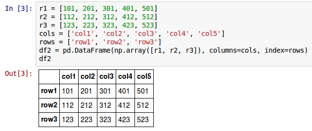
To create a simple 3-rows by 5-columns DataFrame called df2 with user specified row and column index labels, invoke the DataFrame constructor as shown below:
r1 = [101, 201, 301, 401, 501]
r2 = [112, 212, 312, 412, 512]
r3 = [123, 223, 323, 423, 523]
cols = ['col1', 'col2', 'col3', 'col4', 'col5']
rows = ['row1', 'row2', 'row3']
df2 = pd.DataFrame(np.array([r1, r2, r3]), columns=cols, index=rows)
The following shows the screenshot of the result in IPython:
To get the total number of elements in the above DataFrame called df2, access the property size as shown below:
df2.size
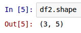
To get the dimensions of the above DataFrame called df2, access the property shape as shown below:
df2.shape
The following shows the screenshot of the result in IPython:
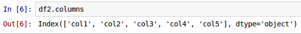
To list all the column index labels from the above DataFrame called df2, access the property columns as shown below:
df2.columns
The following shows the screenshot of the result in IPython:
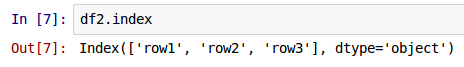
To list all the row index labels from the above DataFrame called df2, access the property index as shown below:
df2.index
The following shows the screenshot of the result in IPython:
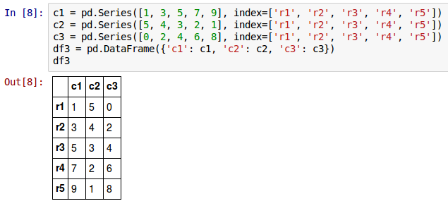
To create a simple 5-rows by 3-columns DataFrame called df3 from a Python dictionary, invoke the DataFrame constructor as shown below:
c1 = pd.Series([1, 3, 5, 7, 9], index=['r1', 'r2', 'r3', 'r4', 'r5'])
c2 = pd.Series([5, 4, 3, 2, 1], index=['r1', 'r2', 'r3', 'r4', 'r5'])
c3 = pd.Series([0, 2, 4, 6, 8], index=['r1', 'r2', 'r3', 'r4', 'r5'])
df3 = pd.DataFrame({'c1': c1, 'c2': c2, 'c3': c3})
The following shows the screenshot of the result in IPython:
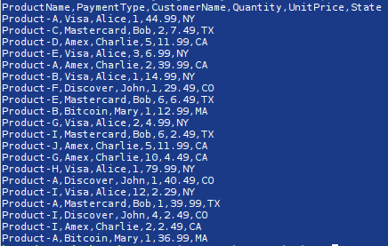
One can also create a DataFrame from a file containing data in a Comma Separated Values (CSV) format.
The following shows the screenshot of a simple data file called transactions.csv containing information for 20 customer transactions, with each transaction represented as 6 fields (columns):
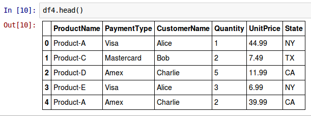
To create a DataFrame called df4 from our sample transactions.csv file, invoke the read_csv() method as shown below:
df4 = pd.read_csv("./transactions.csv")
To take a peek at the top few rows from the above DataFrame called df4, invoke the head() method as shown below:
df4.head()
The following shows the screenshot of the result in IPython:
To take a peek at the last few rows from the above DataFrame called df4, invoke the tail() method as shown below:
df4.tail()
The following shows the screenshot of the result in IPython:

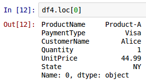
To look-up a row using the row index label 0 from the above DataFrame called df4, one can use the property loc as shown below:
df4.loc[0]
The following shows the screenshot of the result in IPython:
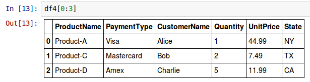
To look-up the first three rows using the row index label from the above DataFrame called df4, one can use the property loc as shown below:
df4[0:3]
The following shows the screenshot of the result in IPython:
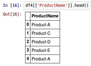
To take a peek at the values of the column with index label ProductName for the top few rows from the above DataFrame called df4, use the syntax as shown below:
df4[['ProductName']].head()
The following shows the screenshot of the result in IPython:
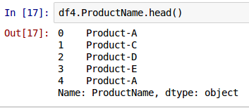
One can also access the same above values for the column with index label ProductName from the above DataFrame called df4 by accessing a dynamically added property with the same name as the column index label using the syntax as shown below:
df4.ProductName.head()
The following shows the screenshot of the result in IPython:
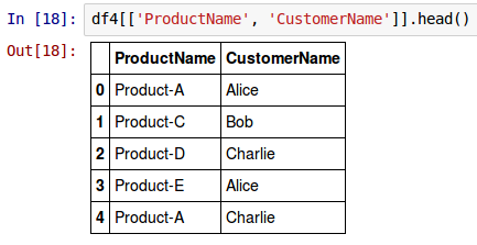
To take a peek at the values of the columns with index labels ProductName and CustomerName for the top few rows from the above DataFrame called df4, use the syntax as shown below:
df4[['ProductName', 'CustomerName']].head()
The following shows the screenshot of the result in IPython:
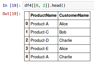
One can also access the same above values for the columns with index labels ProductName and CustomerName using the built-in position indices (which starts with a zero for the first column) for the top few rows from the above DataFrame called df4, use the syntax as shown below:
df4[[0, 2]].head()
The following shows the screenshot of the result in IPython:
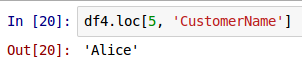
To access the value at the first row index label and the column with index label CustomerName for the top few rows from the above DataFrame called df4, use the syntax as shown below:
df4.loc[5, 'CustomerName']
The following shows the screenshot of the result in IPython:
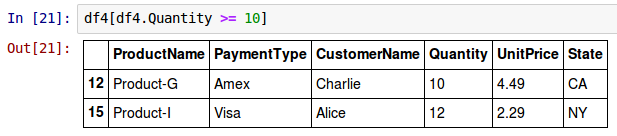
One can filter and select rows from a given DataFrame using logical expressions. For example, to select all the rows for which the column Quantity is greater than or equal to 10 from the above DataFrame called df4, use the syntax as shown below:
df4[df4.Quantity >= 10]
The following shows the screenshot of the above two results in IPython:
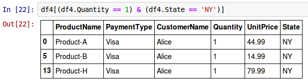
To select all the rows for which the column Quantity is equal to 1 and the column State is equal to NY from the above DataFrame called df4, use the syntax as shown below:
df4[(df4.Quantity == 1) & (df4.State == 'NY')]
The following shows the screenshot of the above two results in IPython:
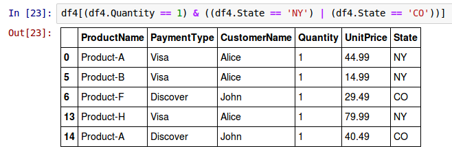
To select all the rows for which the column Quantity is equal to 1 and the column State is equal to NY or CO from the above DataFrame called df4, use the syntax as shown below:
df4[(df4.Quantity == 1) & ((df4.State == 'NY') | (df4.State == 'CO'))]
The following shows the screenshot of the above two results in IPython:
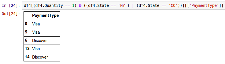
To select only the column PaymentType for all the rows for which the column Quantity is equal to 1 and the column State is equal to NY or CO from the above DataFrame called df4, use the syntax as shown below:
df4[(df4.Quantity == 1) & ((df4.State == 'NY') | (df4.State == 'CO'))][['PaymentType']]
The following shows the screenshot of the above two results in IPython:
To create a new DataFrame called df5 from the existing DataFrame called df4, invoke the method copy() as shown below:
df5 = df4.copy()
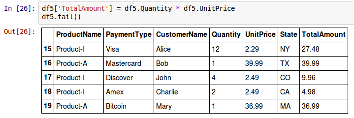
To append a new column called TotalAmount (whose value is the product of columns Quantity and UnitPrice) to the end of all the rows in the above DataFrame called df5, use the syntax as shown below:
df5['TotalAmount'] = df5.Quantity * df5.UnitPrice
The following shows the screenshot of the above two results in IPython:
Let us create a new DataFrame called df6 from the existing DataFrame called df4 as shown below:
df6 = df4.copy()
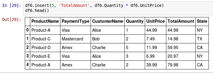
To insert a new column called TotalAmount (whose value is the product of columns Quantity and UnitPrice) as the 6th column after the column UnitPrice and before the column State to all the rows in the above DataFrame called df6, use the syntax as shown below:
df6.insert(5, 'TotalAmount', df6.Quantity * df6.UnitPrice)
The following shows the screenshot of the above two results in IPython:
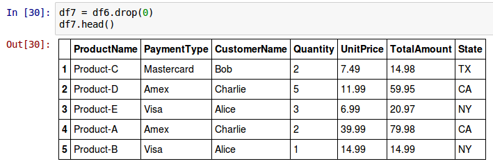
To delete the first row using the row index label from the above DataFrame called df6, invoke the drop() method as shown below:
df7 = df6.drop(0)
The drop() method does not modify the DataFrame on which its invoked. Instead returns a new DataFrame with the actual modification.
The following shows the screenshot of the above two results in IPython:
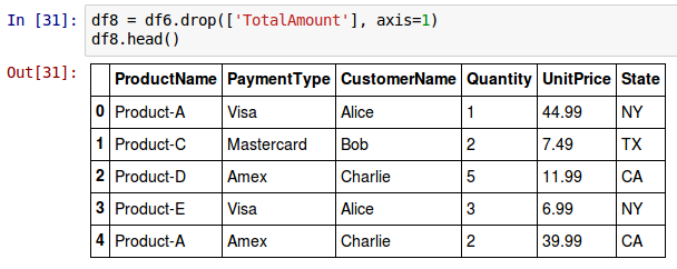
To delete an entire column called TotalAmount from the above DataFrame called df6, invoke the drop() method as shown below:
df8 = df6.drop(['TotalAmount'], axis=1)
Notice the use of the additional axis argument with a value of 1 to specify we want to drop a column. The drop() method does not modify the DataFrame on which its invoked. Instead returns a new DataFrame with the actual modification.
The following shows the screenshot of the above two results in IPython:
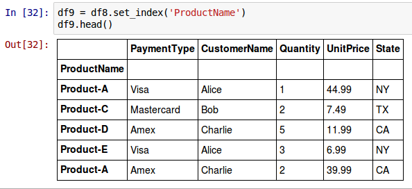
Until now we relied on the default built-in row index labels to access rows in a DataFrame. What if we wanted a real column to serve as the row index ? To select the column ProductName as the new row index label on a DataFrame called df8, invoke the set_index() method as shown below:
df9 = df8.set_index('ProductName')
The set_index() method does not modify the DataFrame on which its invoked. Instead returns a new DataFrame with the actual modification.
The following shows the screenshot of the above two results in IPython:
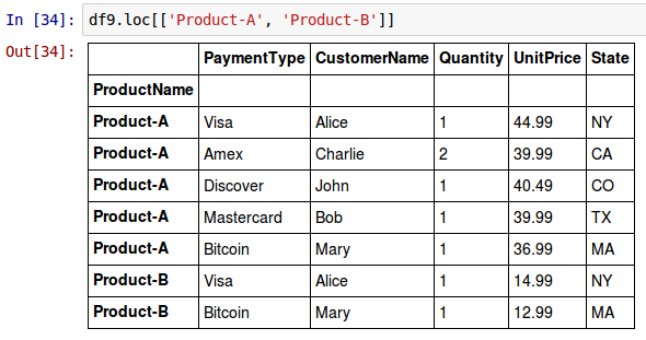
To select all the rows with row index labels equals Product-A and Product-B from the DataFrame called df9, use the syntax as shown below:
df9.loc[['Product-A', 'Product-B']]
The following shows the screenshot of the above two results in IPython:
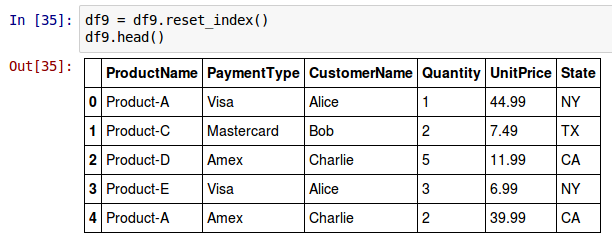
To revert back to the default built-in row index labels to access rows in the DataFrame called df9, invoke the reset_index() method as shown below:
df9 = df9.reset_index()
The reset_index() method does not modify the DataFrame on which its invoked. Instead returns a new DataFrame with the actual modification.
The following shows the screenshot of the above two results in IPython:
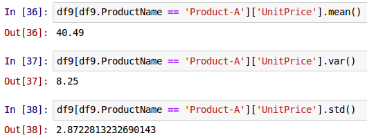
One can perform statistical operations such as finding the mean, the variance, and the standard deviation on a numeric column from the DataFrame called df9 as shown below:
df9[df9.ProductName == 'Product-A']['UnitPrice'].mean()
df9[df9.ProductName == 'Product-A']['UnitPrice'].var()
df9[df9.ProductName == 'Product-A']['UnitPrice'].std()
The following shows the screenshot of the result in IPython:
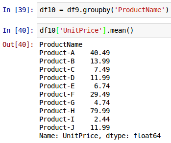
Just like with database tables, one can perform group-by operation on a DataFrame to aggregate and summarize data in columns. To perform a group-by on the column ProductName and find the average (mean) UnitPrice by ProductName on the DataFrame called df9, use the syntax as shown below:
df10 = df9.groupby('ProductName')
df10['UnitPrice'].mean()
The following shows the screenshot of the result in IPython:
We will now create two DataFrame called df11 and df12 as shown below:
r1 = [10, 20, 30, 40, 50]
r2 = [22, 33, 44, 55, 66]
r3 = [36, 48, 54, 72, 84]
cols1 = ['c1', 'c2', 'c3', 'c4', 'c5']
rows1 = ['r1', 'r2', 'r3']
df11 = pd.DataFrame(np.array([r1, r2, r3]), columns=cols1, index=rows1)
r4 = [5, 10, 15, 20]
r5 = [10, 15, 20, 25]
cols2 = ['c1', 'c2', 'c3', 'c4']
rows2 = ['r1', 'r2']
df12 = pd.DataFrame(np.array([r4, r5]), columns=cols2, index=rows2)
One can perform basic arithmetic operations such as addition, subtraction, multiplication, or division on the two DataFrame called df11 and df12. The following example is the subtraction operation:
df11 - df12
Here is another example of dividing the DataFrame called df12 by 5:
df12 / 5
The following shows the screenshot of the result in IPython:
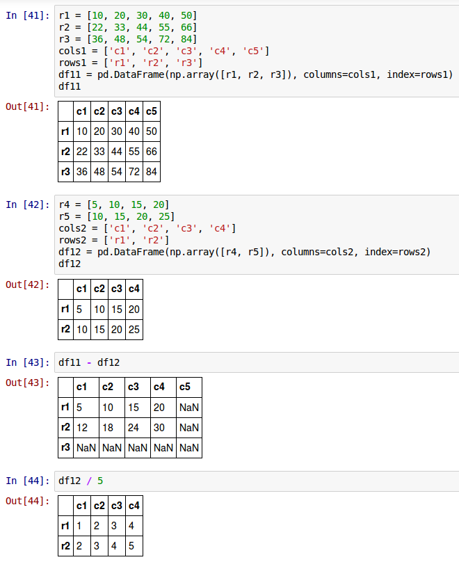
As can be seen from Fig.50 above, DataFrame performs automatic aligment on row and column indices and then performs the arithmetic operation on the matched indices. If either the row or column index is missing from one of the two DataFrames, that result is marked as NaN (Not a Number).
References