Figure.1
Introduction to IPython Notebook
| Bhaskar S | 09/06/2015 |
Overview
IPython Notebook is a feature rich, browser based, interactive computational environment in which one could write and execute Python code, plot graphs, add descriptive text and media.
IPython Notebook is a web-based application that provides scientists and analysts with an agile development tool for both exploratory scientific computation and data analysis.
It records all the inputs and outputs (including descriptive text and media) from the exploratory research in a text document called a Notebook (saved as JSON text) that can be shared with others to reproduce the research work.
Installation and Setup
To make it easy and simple, we choose the open-source Anaconda Python distribution, which includes all the necessary Python packages for science, math, & engineering computations as well as statistical data analysis.
Download the Python 3 version of the Anaconda distribution.
Extract the downloaded archive to a directory, say, /home/abc/anaconda3.
Finally, update the PATH environment variable to include /home/abc/anaconda3/bin.
Using IPython Notebook
Basics
Let /home/abc/ipynb be the directory where we want to save all our work with the IPython Notebook environment.
Open a terminal and ensure we are in the directory /home/abc/ipynb.
To start the IPython Notebook environment, execute the following command:
ipython notebook
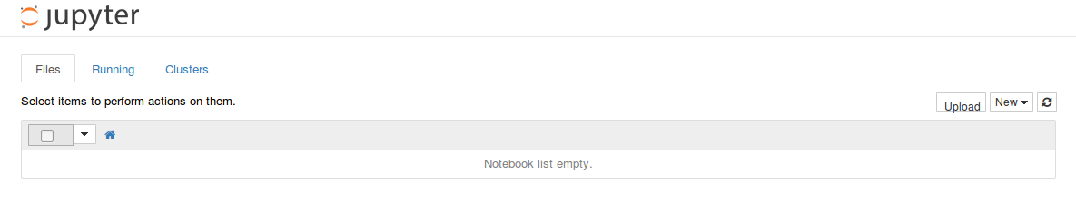
This will launch a web browser as shown in Figure.1 below:
An IPython Notebook is basically a text file (with a .ipynb extension) that has a record of all interactions, including the various code input and their respective execution outputs plus the graph plots, descriptive texts and images.
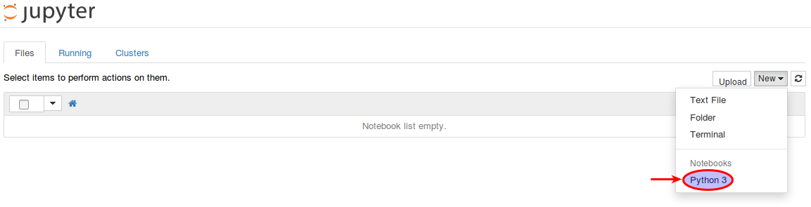
To create a new IPython Notebook, click on the drop-down labeled New on the top right-hand corner and click on the item labelled Python 3 as shown in Figure.2 below:
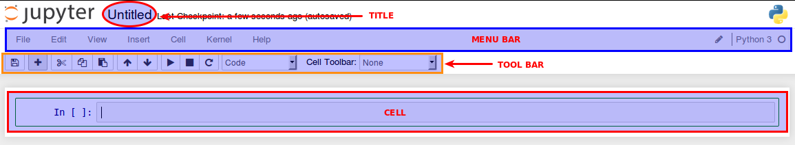
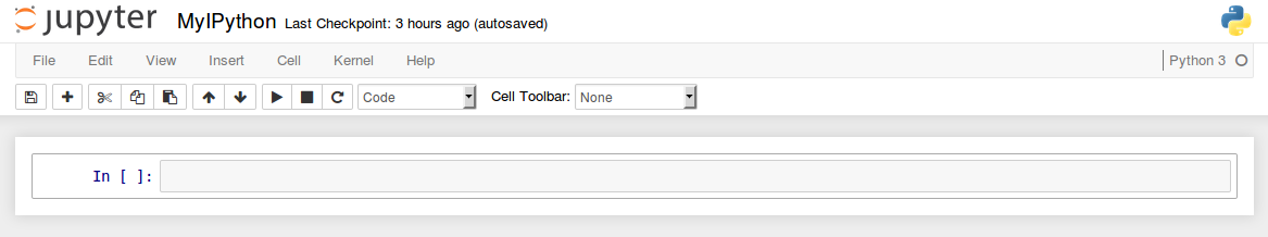
When a new IPython Notebook is created, it is named as Untitled and the title (or name) appears on the top (first) row of the user interface. The second row on the user interface contains a menubar with various options to manipulate the way the notebook functions. The third row on the user interface presents a toolbar that gives quick access to the most commonly used operations within the notebook. Finally, there is the row with an empty text-box labeled In [ ]: where one enters either code or descriptive text and is referred to as a Cell. The Figure.3 below shows the various user interface elements:
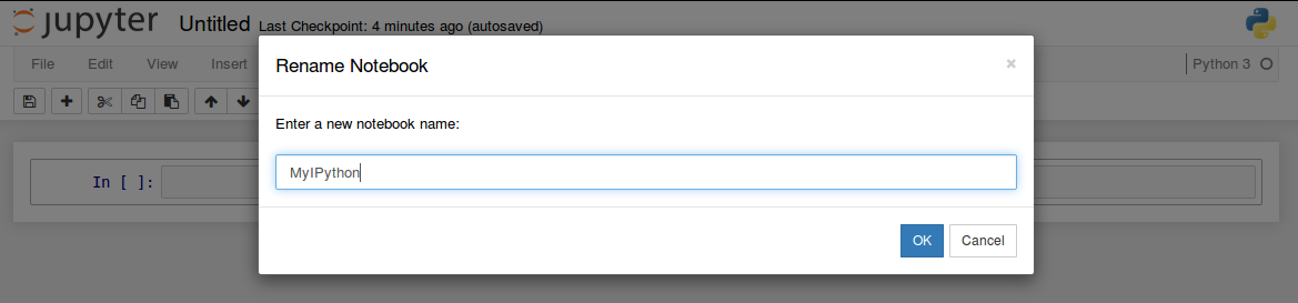
To change the title (or name) to MyIPython, click on the title Untitled and it will pop-up a dialog box to enter a new name as shown in Figure.4 below:
Command Mode
Pressing the Esc key puts the user interface in the Command mode. In the Command mode, the whole notebook user interface comes into focus and the cells have a gray rectangle around them. In this mode, one can perform operations relating to the notebook, such as creating, copying, cutting, moving, or pasting cells. The Figure.5 below shows the user interface in the Command mode:
In the Command mode, one can press certain shortcut keys to emulate actions from the menubar. The following table lists some of the shortcut keys and their action description:
| Shortcut Key | Action Description |
|---|---|
| a | Insert an empty cell above |
| b | Insert an empty cell below |
| c | Copy the cell contents |
| d + d (Press d twice) | Delete the current cell |
| s | Save the notebook |
| v | Paste the cell contents |
| x | Cut the cell contents |
| z | Undo last operation |
| ctrl + j | Move the cell down |
| ctrl + k | Move the cell up |
Edit Mode
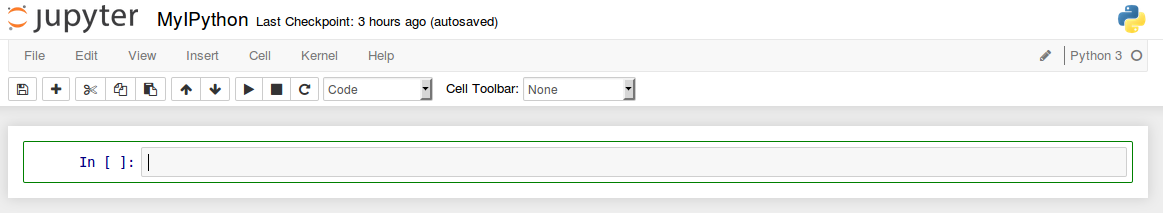
Pressing the Enter key puts the user interface in the Edit mode. In the Edit mode, a single cell has the focus (with a green rectangle around it) and one can perform cell operations such as editing the text or executing code. The Figure.6 below shows the user interface in the Edit mode:
A Notebook is nothing more than a sequence of cells. A cell is a text-box field that can contain multiple lines of text. The text can be Python code or any descriptive rich text.
To execute the contents in a cell, one can choose the menu item Cell->Run or click on the Play icon from the toolbar or press Crtl+Enter or Shift+Enter.
Pressing Crtl+Enter executes the lines in a cell and the focus stays in that cell, while pressing Shift+Enter will execute the lines in a cell and move to the next cell (if one exists) or creates a new empty cell.
Cell Types
A cell can be any one of the following four types:
Code :: A Code cell can contain multiple lines of Python code which can be executed
Markdown :: A Markdown cell can contain multiple lines of descriptive text with special annotations called Markdown language. The Markdown language provides simple text markup syntax to specify which parts of the text should be shown in italics or bold, show lists, etc.
Raw :: A Raw cell can contain multiple lines of text that can be output directly without any execution by the notebook
Heading :: A Heading cell can contain text with different levels of headings. There are 6 levels of headings available - from level 1 (top level) down to level 6 (paragraph). These can be used for creating structured content such as tables of contents, etc
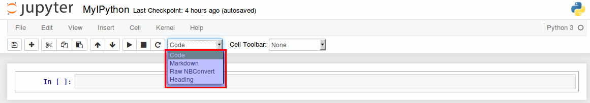
The Figure.7 below shows the way to select the cell type from the drop-down in toolbar of the user interface:
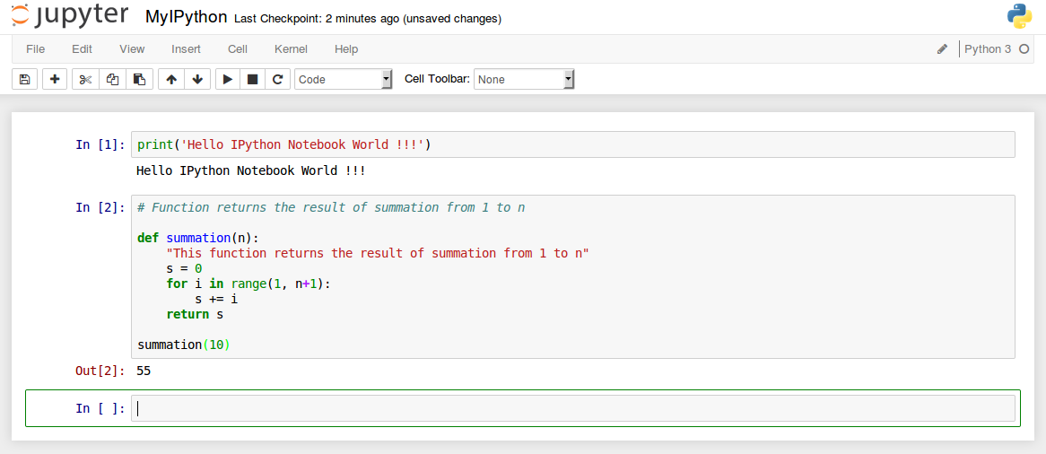
Code Cell
The default cell type is Code. One can enter Python code in a code cell and execute it by pressing Ctrl+Enter. The Figure.8 below shows the user interface after the execution of a simple one line Python code:
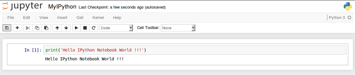
The result is displayed below the code cell.
One can also enter more complex Python code in a code cell and execute it by pressing Shift+Enter. The Figure.9 below shows the user interface after the execution of the complex Python code:
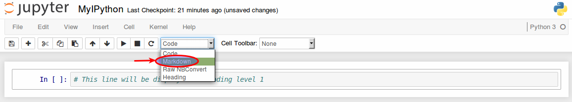
Markdown Cell
To change the cell type to Markdown, choose the Markdown option from the first drop-down list in the toolbar (the default choice is Code).
The Figure.10 below shows the way to select the Markdown cell type from the first drop-down in toolbar of the user interface:
There are 6 levels of paragraph headers.
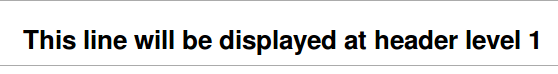
If a Markdown cell, has the following content:
# This line will be displayed at header level 1
It will be displayed at the first header level. Notice the one # (hash) symbol preceding the text.
The Figure.11 below shows how the Markdown cell is rendered:
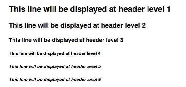
Text preceded by two hashes (##) is displayed at the second header level, three hashes (###) is displayed at the third header level and so on till six hashes (######).
The Figure.12 below shows how the various header Markdown cells are rendered:
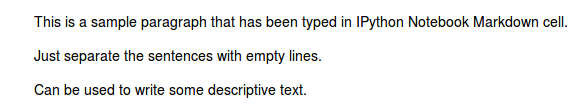
To create a paragraphs, just type the desired text separating them with empty lines as shown below:
          This is a sample paragraph that has been typed in IPython Notebook Markdown cell.

          Just separate the sentences with empty lines.

          Can be used to write some descriptive text.
The Figure.13 below shows how the paragraph Markdown is rendered:
To make some text in italics, surround it with either a single * (star) or an _ (underscore) at the start and end as shown below:
Here is the word in *italics* (or _ITALICS_).
To make some text in bold, surround it with either a double ** (star) or double __ (underscore) at the start and end as shown below:
Here is the word in **bold** (or __BOLD__).
To strike-through some text, surround it with a double ~~ (tilde) at the start and end as shown below:
Here is the word that is ~~Strike Through~~.
The Figure.14 below shows how the various emphasis Markdown texts are rendered:

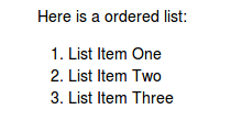
To make an ordered list, enter the text as shown below:
        Here is a ordered list:

        1. List Item One
        2. List Item Two
        3. List Item Three
The Figure.15 below shows how the ordered list Markdown is rendered:
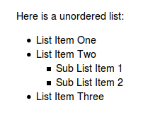
To make an unordered list, enter the text as shown below:
        Here is a unordered list:

        * List Item One
        * List Item Two
            - Sub List Item 1
            - Sub List Item 2
        * List Item Three
The Figure.16 below shows how the unordered list Markdown is rendered:
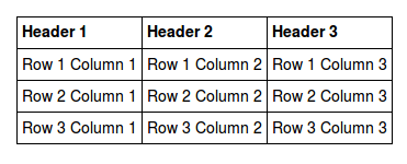
To create a table, enter the text as shown below:
          Header 1 | Header 2 | Header 3
          ---------|----------|---------
          Row 1 Column 1 | Row 1 Column 2 | Row 1 Column 3
          Row 2 Column 1 | Row 2 Column 2 | Row 2 Column 3
          Row 3 Column 1 | Row 3 Column 2 | Row 3 Column 3
The Figure.17 below shows how the table Markdown is rendered:
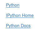
To create URL links, enter the text as shown below:
          [Python](http://www.python.org)

          [IPython Home](http://www.ipython.org)

          [Python Docs](http://docs.python.org)
The Figure.18 below shows how the links Markdown is rendered:
To create a horizontal line, enter the text (three dashes) as shown below:
---
The Figure.19 below shows how the horizontal line Markdown is rendered:

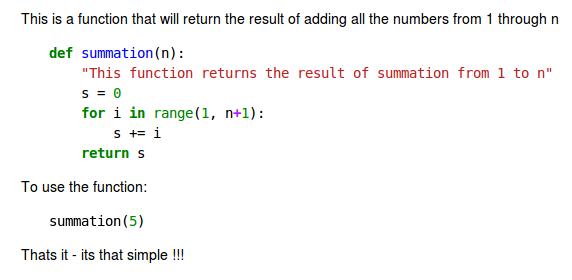
To document Python code, enter the text as shown below:
          This is a function that will return the result of adding all the numbers from 1 through n

          ```python
          def summation(n):
              "This function returns the result of summation from 1 to n"
              s = 0
              for i in range(1, n+1):
                  s += i
              return s
          ```

          To use the function:

          ```python
          summation(5)
          ```

          Thats it - its that simple !!!
Code to be documented must be preceded by the three backquotes followed by the word python and ending with the three backquotes.
The Figure.20 below shows how the Python code Markdown is rendered:
Built-in Magic Commands
The IPython Notebook magic functions are built-in commands that perform certain actions on execution.
To list all the magic command built into IPython Notebook, execute the following command in a code cell:
%lsmagic
The Figure.21 below shows the results of the execution:
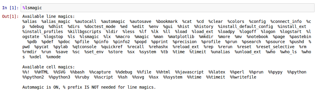
From the output in the Figure.21 above, we can see that we have two types of magic commands:
With Prefix % :: referred to as Line Magics, they get the rest of the line as an argument
With Prefix %% :: referred to as Cell Magics, they not only get the rest of the line as an argument, but also the each line below as a separate arguments
We will explore only some of the commonly used magic commands in the following paragraphs.
The following table lists the common OS level commands as line magic comnmands:
| Shortcut Key | Action Description |
|---|---|
| %cat | Display the contents of a file |
| %cd | Change the specified directory |
| %cp | Copy a source file to a target file |
| %env | To get or list environment variables |
| %less | Display the contents of the specified file through a pager |
| %ls | List the contents of the current working directory |
| %mkdir | Create the specified directory in the current working directory |
| %more | Display the contents of the specified file through a pager |
| %mv | Rename a file or a directory |
| %pwd | Display the name of the current working directory |
| %rm | Delete the specified file |
| %rmdir | Delete the specified directory |
| %set_env | Set the environment variable |
Note that the IPython Notebook is an interactive platform. All the variables or functions defined in an interactive session are alive until the session is terminated.
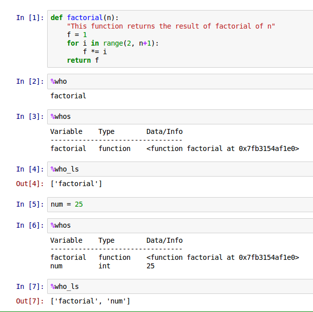
To list all the variables/functions in an interactive session, execute the following magic command in a code cell:
%who
To list all the variables/functions in an interactive session in a sorted order, execute the following magic command in a code cell:
%who_ls
To list all the variables/functions in an interactive session with additional information, execute the following magic command in a code cell:
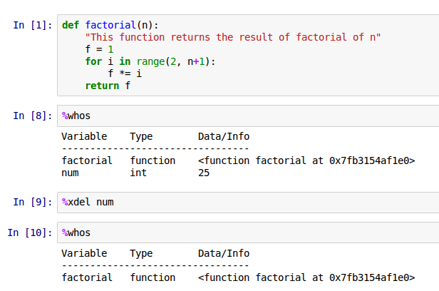
%whos
The Figure.22 below shows the results of the various magic command executions:
To delete a variable/function in an interactive session, execute the following magic command in a code cell:
%xdel num
The Figure.23 below shows the results of the various magic command executions:
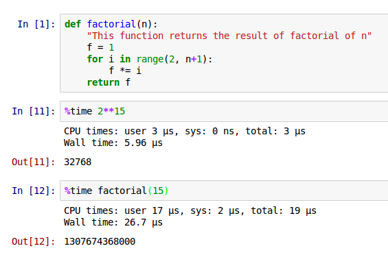
To determine the execution time of a Python expression, execute the following magic command in a code cell:
%time 2**15
To determine the execution time of a Python statement, execute the following magic command in a code cell:
%time factorial(15)
The Figure.24 below shows the results of the various magic command executions:
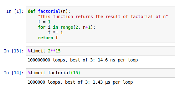
One can also determine the execution time of a Python expression or statement using the %timeit magic command.
It is similar to the %time magic command except that it runs few iterations and reports the average of the best of three iterations.
The Figure.25 below shows the results of the various magic command executions:
References