Figure.1
| PolarSPARC |
Machine Learning - Linear Regression - Part 1
| Bhaskar S | 03/19/2022 |
Overview
Regression is a statistical process, which attempts to determine the relationship between a dependent outcome (or a response) variable, typically denoted using the letter $y$, and one or more independent feature variables, typically denoted using letters $x_1, x_2, ..., x_n$, etc.
Linear Regression is applicable when the Dependent Outcome (sometimes called a Response or a Target) variable is a CONTINUOUS variable and has a linear relationship with one or more Independent Feature (or Predictor) variable(s).
In general, one could express the relationship between the dependent outcome variable and the independent feature variables in mathematical terms as $y = \beta_0 + \beta_1.x_1 + ... + \beta_n.x_n$, where coefficients $\beta_1, \beta_2, ..., \beta_n$ are referred to as the Regression Coefficients (or the weights or the parameters) associated with the corresponding independent variables $x_1, x_2, ..., x_n$ and $\beta_0$ is a constant.
In other words, $y = \beta_0 + \sum_{i=1}^n \beta_i.x_i$
The process of determining the coefficients (or the weights or the parameters) of the linear regression equation is often referred to as the Ordinary Least Squares (or OLS).
Simple Linear Regression
In the case of Simple Linear Regression, there is ONE dependent outcome variable, that has a relationship with ONE independent feature variable.
To understand simple linear regression, let us consider the simple case of predicting (or estimating) a dependent outcome variable $y$ using a single independent feature variable $x$. For every value of the independent feature variable $x$, there is a corresponding outcome value $y$. That is, we will have a set of pairs $[(x_0, y_0), (x_1, y_1), ..., (x_n, y_n)]$.
In other words, one could estimate the dependent outcome value using the model $\hat{y} = \beta_0 + \beta_1.x$. Notice that this equation is similar to that of a line $y = m.x + b$, where $m$ is the Slope of the line and $b$ is the Intercept of the line. Hence, the model for simple linear regression is often times referred to as the Line of Best Fit.
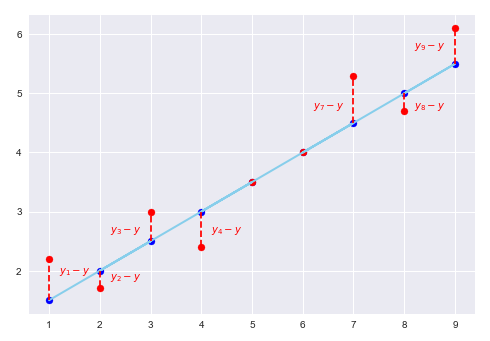
Consider the following plot that illustrates the line of best fit, the actual outcome values (red dots), and the estimated (or predicted) outcome values (blue dots):
For the line of best fit, the idea is to minimize the sum of all the residual distances (or the errors) between the actual values of the outcome variable (red dots) $y_i$ compared to their predicted values (blue dots) $\hat{y_i}$.
In mathematical terms, the sum of all the residual errors can be represented as $E = \sum_{i=1}^n (y_i - \hat{y_i})$. However, since some residuals will be POSITIVE and others NEGATIVE, the result of their sum will end up cancelling each other and we end up with $E = 0$, which is not correct. To avoid this, we need to sum the SQUARE of the residual errors. In other words, $E = \sum_{i=1}^n (y_i - \hat{y_i})^2$. This equation is often referred to as the Sum of Squared Errors (or SSE) or Residual Sum of Squares (or RSS).
For the optimal line of best fit, we need to minimize the Error Function (or the Cost Function) $E = \sum_{i=1}^n (y_i - \hat{y_i})^2 = \sum_{i=1}^n (y_i - (\beta_0 + \beta_1.x_i))^2$.
We know the values for $x_i$ and $y_i$, but have two unknown variables $\beta_0$ and $\beta_1$.
In order to MINIMIZE the error $E$, we need to take the partial derivatives of the error function with respect to the two unknown variables $\beta_0$ and $\beta_1$ and set their result to zero.
In other words, we need to solve for $\Large{\frac{\partial{E}}{\partial{\beta_0}}}$ $= 0$ and $\Large{\frac{\partial{E}} {\partial{\beta_1}}}$ $= 0$.
First, $\Large{\frac{\partial{E}}{\partial{\beta_0}}}$ $= \sum_{i=1}^n 2(y_i - (\beta_0 + \beta_1.x_i)) (-1)$
On simplification, we get, $- \sum_{i=1}^n y_i + \beta_0 \sum_{i=1}^n 1 + \beta_1 \sum_{i=1}^n x_i = 0$
Or, $\sum_{i=1}^n y_i = \beta_0 n + \beta_1 \sum_{i=1}^n x_i$ ..... $\color{red} (1)$
Second, $\Large{\frac{\partial{E}}{\partial{\beta_1}}}$ $= \sum_{i=1}^n 2(y_i - (\beta_0 + \beta_1.x_i)) (-x_i)$
On simplification, we get, $- \sum_{i=1}^n x_i.y_i + \beta_0 \sum_{i=1}^n x_i + \beta_1 \sum_{i=1}^n x_i^2 = 0$
Or, $\sum_{i=1}^n x_i.y_i = \beta_0 \sum_{i=1}^n x_i + \beta_1 \sum_{i=1}^n x_i^2$ ..... $\color{red} (2)$
Let $A = \sum_{i=1}^n x_i^2$, $B = \sum_{i=1}^n x_i$, $C = \sum_{i=1}^n x_i.y_i$, and $D = \sum_{i=1}^n y_i$
Therefore, equations $\color{red} (1)$ and $\color{red} (2)$ can be rewritten as follows:
$D = \beta_0 n + \beta_1 B$ ..... $\color{red} (1)$
$C = \beta_0 B + \beta_1 A$ ..... $\color{red} (2)$
Solving equations $\color{red} (1)$ and $\color{red} (2)$, we get the following:
$\beta_0 = \Large{\frac{(CB - DA)}{(B^2 - nA)}}$ $= \Large{\frac{(DA - CB)}{(nA - B^2)}}$ $= \Large{\frac{\sum y_i \sum x_i^2 - \sum x_i \sum x_i.y_i}{n \sum x_i^2 - (\sum x_i)^2}}$ ..... $\color{red} (3)$
$\beta_1 = \Large{\frac{(nC - DB)}{(nA - B^2)}}$ $= \Large{\frac{n \sum x_i.y_i - \sum x_i \sum y_i}{n \sum x_i^2 - (\sum x_i)^2}}$ ..... $\color{red} (4)$
We know the following:
$\bar{x} =$ $\Large{\frac{1}{n}}$ $\sum_{i=1}^n x_i$
$\bar{y} =$ $\Large{\frac{1}{n}}$ $\sum_{i=1}^n y_i$
$\overline{xy} =$ $\Large{\frac{1}{n}}$ $\sum_{i=1}^n x_i.y_i$
Diving both the equations $\color{red} (3)$ and $\color{red} (4)$ by $n^2$ and simplifying, we will arrive at the following results:
$\color{red} \boldsymbol{\beta_0}$ $= \bbox[pink,2pt]{\Large{\frac{\bar{y}.\bar{x^2} - \bar{x}.\overline{xy}}{\bar{x^2} - \bar{x}^2}}}$
$\color{red} \boldsymbol{\beta_1}$ $= \bbox[pink,2pt]{\Large{\frac{\overline{xy} - \bar{x}.\bar{y}}{\bar{x^2} - \bar{x}^2}}}$
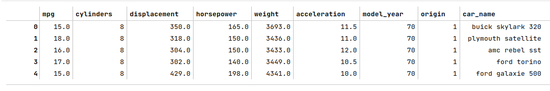
Let us use the Auto MPG dataset to demonstrate the relationship between the Horsepower and the MPG.
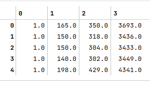
The following illustration shows the first 5 rows of the auto mpg dataset:
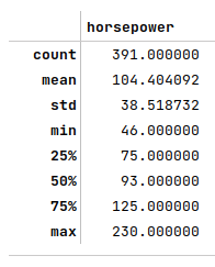
The following illustration shows the summary statistics of the auto horsepower feature variable):
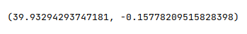
The following illustration shows the values of $\beta_0$ and $\beta_1$ computed using the equations derived above:
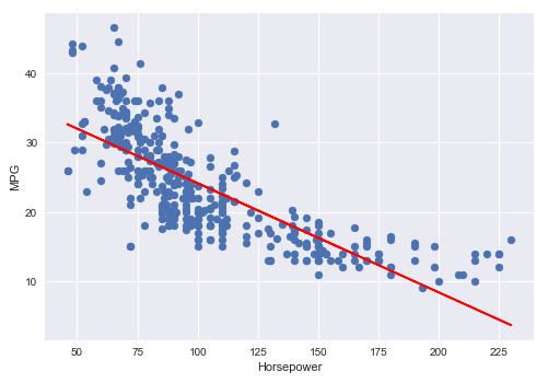
The following illustration shows the scatter plot between the auto horsepower feature variable and the auto mpg outcome variable, along with the line of best fit using the derivation for $\beta_0$ and $\beta_1$:
Multiple Linear Regression
In the case of Multiple Linear Regression, there is ONE dependent outcome variable that has relationships with MORE than ONE independent feature variables.
To understand multiple linear regression, let us consider the case of predicting (or estimating) a dependent variable $y$ using $n$ independent feature variables $x_1, x_2, ..., x_n$. In mathematical terms, one could estimate the dependent outcome value using the linear model $\hat{y} = \beta_0 + \beta_1.x_1 + \beta_2.x_2 + ... + \beta_n.x_n$.
Using the matrix notation, one could write the above linear model as: $\hat{y} = \beta_0 + \begin{bmatrix} \beta_1 & \beta_2 & ... & \beta_n \end{bmatrix} \begin{bmatrix} x_1 \\ x_2 \\ ... \\ x_n \end{bmatrix}$
That is, $\hat{y} = \begin{bmatrix} \beta_0 & \beta_1 & ... & \beta_n \end{bmatrix} \begin{bmatrix} 1 \\ x_1 \\ x_2 \\ ... \\ x_n \end{bmatrix}$.
Now, what about extending the above linear model to predict $m$ dependent output values ???
In other words, $y_m = \begin{bmatrix} y_1 \\ y_2 \\ ... \\ y_m \end{bmatrix}$
Then, $\begin{bmatrix} y_1 \\ y_2 \\ ... \\ y_m \end{bmatrix} = \begin{bmatrix} 1 & x_{1,1} & x_{1,2} & ... & x_{1,n} \\ 1 & x_{2,1} & x_{2,2} & ... & x_{2,n} \\ ... & ... & ... & ... & ... \\ 1 & x_{m,1} & x_{m,2} & ... & x_{m,n} \end{bmatrix} \begin{bmatrix} \beta_0 \\ \beta_1 \\ ... \\ \beta_n \end{bmatrix}$
Once again, using the matrix notation, we arrive at $\hat{y} = X\beta$, where $X$ is a matrix. Note that $\beta$ has to be to the right of $X$ in order to apply the coefficients (or weights) appropriately to each row (one set of feature values) of $X$.
Given that we desire to predict $m$ dependent output values, for the optimal line of best fit, we need to minimize $E = \sum_{i=1}^m (y_i - \hat{y_i})^2$.
Using the matrix notation, $E = \begin{bmatrix} (y_1-\hat{y_1}) & (y_2-\hat{y_2}) & ... & (y_m-\hat{y_m}) \end{bmatrix} \begin{bmatrix} (y_1-\hat{y_1}) \\ (y_2-\hat{y_2}) \\ ... \\ (y_m-\hat{y_m}) \end{bmatrix}$
If $y = \begin{bmatrix} y_1 \\ y_2 \\ ... \\ y_m \end{bmatrix}$ and $\hat{y} = \begin{bmatrix} \hat{y_1} \\ \hat{y_2} \\ ... \\ \hat{y_m} \end{bmatrix}$, then $\begin{bmatrix} (y_1-\hat{y_1}) \\ (y_2-\hat{y_2}) \\ ... \\ (y_m-\hat{y_m}) \end{bmatrix} = \begin{bmatrix} y_1 \\ y_2 \\ ... \\ y_m \end{bmatrix} - \begin{bmatrix} \hat{y_1} \\ \hat{y_2} \\ ... \\ \hat{y_m} \end{bmatrix} = y - \hat{y}$
Therefore, $E = (y - \hat{y})^T(y - \hat{y}) = (y^T - \hat{y}^T)(y - \hat{y}) = (y^T - (X\beta)^T)(y - X\beta) = (y^T - \beta^TX^T)(y - X\beta)$.
That is, $E = y^Ty - \beta^TX^Ty - y^TX\beta + \beta^TX^TX\beta$.
$(X\beta)^T = \beta^TX^T$
We know $(y^TX\beta)^T = \beta^TX^Ty$ and $y^TX\beta$ is a scalar. This implies that the transpose of the scalar is the scalar itself. Hence, $y^TX\beta$ can be substituted with $\beta^TX^Ty$.
Therefore, $E = y^Ty - 2\beta^TX^Ty + \beta^TX^TX\beta$.
In order to MINIMIZE the error $E$, we need to take the partial derivatives of the error function with respect to $\beta$ and set the result to zero.
In other words, we need to solve for $\Large{\frac{\partial{E}}{\partial{\beta}}}$ $= 0$.
1. $\Large{\frac{\partial}{\partial{\beta}}}$ $y^Ty = 0$
2. $\Large{\frac{\partial}{\partial{\beta}}}$ $\beta^TX^Ty = X^Ty$
3. $\Large{\frac{\partial}{\partial{\beta}}}$ $y^TX\beta = y^TX$
4. $\Large{\frac{\partial}{\partial{\beta}}}$ $\beta^TX^TX\beta = 2X^TX\beta$
Therefore, $\Large{\frac{\partial{E}}{\partial{\beta}}}$ $= 0 - 2X^Ty + 2X^TX\beta$
That is, $\Large{\frac{\partial{E}}{\partial{\beta}}}$ $= - 2X^Ty + 2X^TX\beta$
To minimize the error, $\Large{\frac{\partial{E}}{\partial{\beta}}}$ $= 0$
That is, $- 2X^Ty + 2X^TX\beta = 0$
Or, $X^TX\beta = X^Ty$
To solve for $\beta$, $(X^TX)^{-1}X^TX\beta = (X^TX)^{-1}X^Ty$
Simplifying, we get the following:
$\color{red} \boldsymbol{\beta}$ $= \bbox[pink,2pt]{(X^TX)^{-1}X^Ty}$
Once again, we use the Auto MPG dataset to demonstrate the relationship between the dependent response variable MPG and the three feature variables - Horsepower, Displacement, and Weight respectively.
The following illustration shows the first 5 rows of the feature variable matrix:
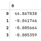
The following illustration shows the $\beta$ values computed using the equation derived above:
Model Evaluation Metrics
In the following paragraphs we will look at the different metrics that help us evaluate the effectiveness of the linear regression model.
Mean Squared Error
Mean Squared Error (or MSE) is a metric that measures the amount of error from the regression model.
In mathematical terms,
$\color{red} \boldsymbol{MSE}$ $= \bbox[pink,2pt]{\Large{\frac{SSE}{n}}}$
where
$SSE = \sum_{i=1}^n (y_i - \hat{y_i})^2$ is called Sum of Squared Errors and represents the variability from the actual expected value.
Root Mean Squared Error
Root Mean Squared Error (or RMSE) is a metric that represents the standard deviation of residuals from the regression model.
In mathematical terms,
$\color{red} \boldsymbol{RMSE}$ $= \bbox[pink,2pt]{\sqrt{MSE}}$
R-Squared
R-Square is a metric (or measure) that evaluates the goodness (or accuracy) of prediction by a regression model. It is often referred to as the Coefficient of Determination and is denoted using the symbol $R^2$.
In other words, $R^2$ represents the proportion of variance of the dependent outcome variable that is influenced (or explained) by the independent feature variable(s) in the regression model.
The $R^2$ value ranges from $0$ to $1$. For example, if $R^2$ is $0.85$, then it indicates that $85%$ of the variation in the response variable is explained by the predictor variables.
In mathematical terms,
$\color{red} \boldsymbol{R^2}$ $= \bbox[pink,2pt]{1 - \Large{\frac{SSE}{SST}}}$
where
$SST = \sum_{i=1}^n (y_i - \bar{y})^2$ is called Sum of Squared Total and represents the total variability from the mean
$SSE = \sum_{i=1}^n (y_i - \hat{y_i})^2$ is called Sum of Squared Errors and represents the variability from the actual expected value.
For a perfectly fit linear regression model, $SSE = 0$ and $R^2 = 1$.
Adjusted R-Squared
When additional independent feature (or predictor) variables that have no influence on the dependent outcome (or response) are added to the regression model, the value of $R^2$ tends to increase and appears to indicate the model is a better fit, when in reality it is NOT and misleading.
The Adjusted R-Square, denoted by $\bar{R}^2$ (or $R_{adj}^2$), addresses the issue by taking into account the number of independent feature variables in the model.
If $p$ is the number independent feature variables, then:
$\color{red} \boldsymbol{\bar{R}^2}$ $= \bbox[pink,2pt]{1 - \Large{\frac{(1 - R^2)(n - 1)}{n - p - 1}}}$
Hands-on Demo
The following are the links to the Jupyter Notebooks that provides an hands-on demo for this article:
References