Machine Learning - Principal Component Analysis using Scikit-Learn

The number of feature variables in a data set used for predicting the target is referred to as the Dimensionality of the data set.

As the number of feature variables in a data set increases, it has some interesting implications, which are as follows:

Need more samples in the data set for better training and testing
Increased complexity of the model that could lead to model overfitting
Hard to explain the model behavior
Increased storage and compute complexity

The task of reducing the number of feature variables from a data set is referred to as Dimensionality Reduction. One of the popular techniques for Dimensionality Reduction is the Principal Component Analysis (or PCA for short).

Principal Component Analysis

In the following sections, we will unravel the idea behind Principal Component Analysis (or PCA) from a geometric point of view for better intuition and understanding.

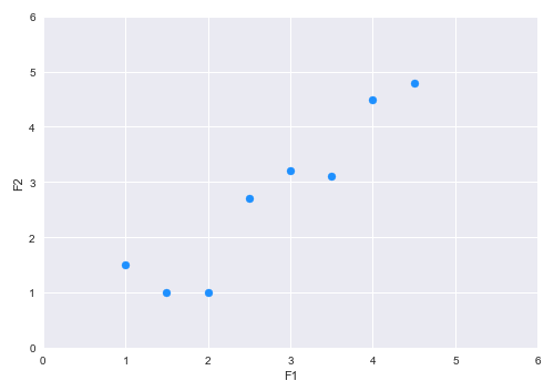
Let us assume a simple hypothetical data set with two feature variables F1 and F2. The following illustration shows the plot of the two features in a two-dimensional space:

Looking at the plot, one can infer that there is a positive relationship between F1 and F2. One can explain this relationship using a vector line. There can be many vector lines in this two-dimensional space - which one do we choose ??? For simplicity, let us just consider the two vector lines - vector $v$ (in red) and vector $w$ (in blue) as shown in the illustration below:

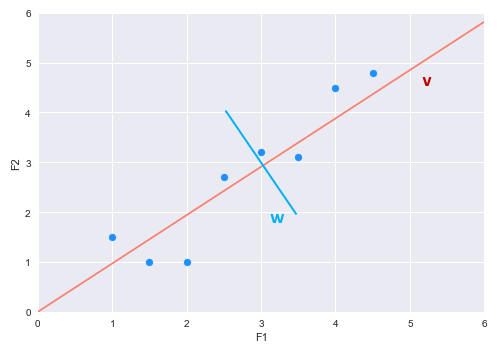
Now, let us look at one of the points (represented as vector $a$) as shown in the illustration below:

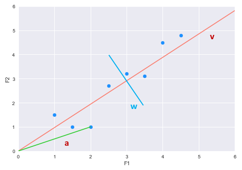
From Linear Algebra, we know the vector $a$ (the point) can be projected onto the vector $v$. The new projected vector (dashed blue line on the vector $v$) will be a scaled version of the vector $v$. The following illustration shows the vector projection:

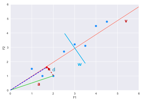
Similarly, we can project the vector $a$ (the point) onto the vector $w$. If we project all the points onto both the vectors $v$ and $w$, we will realize that the variation of the points on vector $v$ is larger (spread out) versus the points on vector $w$ (squished). This implies that with the projections onto vector $w$, there will be some information loss (some points will overlap). Hence, the idea is to pick the vector line with maximum variance (vector $v$ in our example) so that we can capture more information about the two features F1 and F2.

The projected vector (dashed blue line on the vector $v$) will be a scaled version of the vector $v$. If $\lambda$ is a scalar, then the projected vector would be $\lambda.v$. How do we find the value for the scalar $\lambda$ ???

Let $d$ be the vector from the head of vector $a$ to the projected point on vector $v$.

Then, $a + d = \lambda.v$

Or, $d = \lambda.v - a$

We know the vectors $d$ and $v$ must be orthogonal, meaning the angle between them must be $90^{\circ}$.

From Linear Algebra, we know the dot product of orthogonal vectors must be zero. That is, $d.v = 0$

That is, $(\lambda.v - a).v = 0$

Or, $\lambda.v.v - a.v = 0$

Rearranging, we get: $\lambda = \Large{\frac{a.v}{v.v}}$

Once again from Linear Algebra, we know: $\lVert v \rVert = \sqrt{v.v}$

Therefore, the equation for $\lambda$ can be written as: $\lambda = \Large{\frac{a.v}{{\lVert v \rVert}^2}}$

Hence, the projected vector $\lambda.v = \Large{\frac{a.v}{{\lVert v \rVert}^2}}$ $.v$

If we continue to project all the points (or vectors) onto the vector $v$, we in effect will transform the two-dimensional coordinate space into a one-dimensional space (a single line). In other words, we have reduced the two features to just one.

This reduction was possible since there was a clear RELATIONSHIP between the two feature variables F1 and F2. This in essence is the idea behind Dimensionality Reduction using PCA.

The following sections we will use a simple example to work through the steps involved in the Principal Component Analysis algorithm:

Consider the following simple data set with 3 feature variables $X_1$, $X_2$, and $X_3$ as shown in the illustration below:

Figure.5
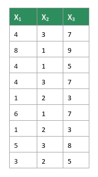
PCA uses the directional relationship between each of the feature variables (covariance) in the data set. In order to compute the covariance, we need to standardize the values of all the feature variables to a common scale. This is achieved by replacing each of the values with its corresponding Z-score.

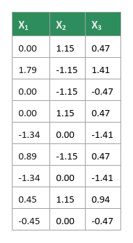
That is, $x_i = \Large{\frac{x_i - \mu}{\sigma}}$, where $\mu$ is the mean and $\sigma$ is the standard deviation.

The following illustration shows the standardized data set:

Figure.6
Create a covariance matrix which captures the directinal relationship between each pair of the feature variables from our data set.

The following illustration shows the template for the covariance matrix with respect to our data set:

Figure.7

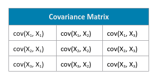
That is, $cov(X, Y) = \Large{\Large{\frac{\sum_{i=1}^n (x_i - \bar{x})(y_i - \bar{y})}{n-1}}}$, where $\bar{x}$ is the mean for feature X and $\bar{y}$ is the mean for feature Y, and $n$ is the number of samples.

The following illustration shows the computed covariance matrix for our data set:

Figure.8
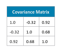
Perform an Eigen Decomposition on the covariance matrix from the previous step. For more details on this topic from Linear Algebra refer to the article Introduction to Linear Algebra - Part 4. The idea is to decompose the covariance matrix to a set of vectors called the Eigen Vectors (represents the projection of the feature relationships) and an associated set of scalars called the Eigen Values (represents the scale or importance of the features). Each of the eigen vectors from the decomposition are referred to as the Principal Components of the original data set.

The following illustration shows the Eigen Vectors and Eigen Values for our covariance matrix:

Figure.9
From the Eigen Values, we can conclude that the principal components corresponding to the feature variables $X_2$ and $X_3$ are more important in our data set. In other words, the principal components corresponding to the feature variables $X_2$ and $X_3$ capture all the information from the data set after dropping the principal component associated to the feature variable $X_1$.

In the following sections, we will demonstrate the use of Principal Component Analysis (using scikit-learn) by leveraging the popular Auto MPG dataset.

The first step is to import all the necessary Python modules such as, pandas and scikit-learn as shown below:

import pandas as pd
from sklearn.preprocessing import StandardScaler
from sklearn.decomposition import PCA
from sklearn.model_selection import train_test_split
from sklearn.linear_model import LinearRegression
from sklearn.metrics import r2_score

The next step is to load the auto mpg data set into a pandas dataframe and assign the column names as shown below:

url = 'https://archive.ics.uci.edu/ml/machine-learning-databases/auto-mpg/auto-mpg.data'
auto_df = pd.read_csv(url, delim_whitespace=True)
auto_df.columns = ['mpg', 'cylinders', 'displacement', 'horsepower', 'weight', 'acceleration', 'model_year', 'origin', 'car_name']

The next step is to fix the data types, drop some unwanted features variables (like model_year, origin, and car_name), and drop the rows with missing values from the auto mpg data set as shown below:

auto_df.horsepower = pd.to_numeric(auto_df.horsepower, errors='coerce')
auto_df.car_name = auto_df.car_name.astype('string')
auto_df = auto_df.drop(['model_year', 'origin', 'car_name'], axis=1)
auto_df = auto_df[auto_df.horsepower.notnull()]
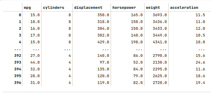
auto_df

The following illustration displays the columns/rows of the auto mpg dataframe:

The next step is to create the training dataset and a test dataset with the desired feature (or predictor) variables. We create a 75% training dataset and a 25% test dataset with the four feature variables acceleration, cylinders, displacement, horsepower, and weight as shown below:

X_train, X_test, y_train, y_test = train_test_split(auto_df[['acceleration', 'cylinders', 'displacement', 'horsepower', 'weight']], auto_df['mpg'], test_size=0.25, random_state=101)

The next step is to create an instance of the standardization scaler to scale the desired feature (or predictor) variables in both the training and test dataframes as shown below:

scaler = StandardScaler()
s_X_train = pd.DataFrame(scaler.fit_transform(X_train), columns=X_train.columns, index=X_train.index)
s_X_test = pd.DataFrame(scaler.transform(X_test), columns=X_test.columns, index=X_test.index)

The next step is to perform the PCA in order to extract the important features from the scaled training and test dataframes as shown below:

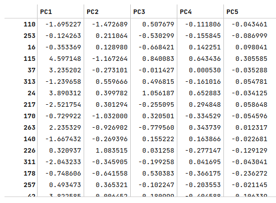
columns = ['PC1', 'PC2', 'PC3', 'PC4', 'PC5']
pca = PCA(random_state=101)
r_X_train = pd.DataFrame(pca.fit_transform(s_X_train), columns=columns, index=s_X_train.index)
r_X_test = pd.DataFrame(pca.transform(s_X_test), columns=columns, index=s_X_test.index)
r_X_train

The following illustration displays the columns/rows from the decomposed principal components:

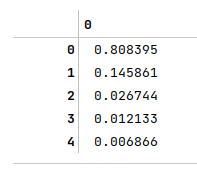
The next step is to display the variance explained by the principal components as shown below:

pca.explained_variance_ratio_

The following illustration displays the variances by each principal component:

Given the first two principal components explain most of the variances from the auto mpg data set, we will use them for in training and testing the regression model as shown below:

drop_columns = ['PC3', 'PC4', 'PC5']
r_X_train2 = r_X_train.drop(drop_columns, axis=1)
r_X_test2 = r_X_test.drop(drop_columns, axis=1)
r_X_train2

The next step is to initialize and train the linear regression model using the dimension reduced training dataframe as shown below:

model = LinearRegression(fit_intercept=True)
model.fit(r_X_train2, y_train)

The next step is to use the trained linear regression model to predict the target (mpg) using the dimension reduced test dataframe as shown below:

y_predict = model.predict(r_X_test2)

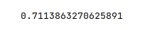
The final step is to display the $R^2$ value for the linear regression model as shown below:

r2_score(y_test, y_predict)

The following illustration displays the $R^2$ value for the model:

The following is the link to the Jupyter Notebook that provides an hands-on demo for this article:

Principal Component Analysis