Apache Spark 2.x Quick Notes :: Part - 2
| Bhaskar S |
*UPDATED*10/05/2019 |
In Part-1 of this
series, we introduced Apache Spark as a general purpose distributed computing engine for data processing on a cluster of
commodity computers.
What does that really mean though ? Let us break it down ...
A Spark cluster consists of a Driver process running within a Master
node and Executor process(es) running within each of the Worker
nodes. When a Spark job is submitted, the Driver partitions and distributes the job as tasks to the Executor process (on
different Worker nodes) for further processing. As the application job executes, the Executor process(es) report back the
state of the task(s) to the Driver process and thus the Driver maintains the overall status of the application job.
Ok - this explains the high-level view of the distributed compute cluster. How does the Driver process know which Executors
are available for processing and whom to distribute the tasks to ? This is where the
Cluster Manager comes into play. The Cluster Manager keeps track of the state of the cluster resources (which
Executor process(es) on which Worker nodes are available, etc).
The Driver process has a connection to the Cluster Manager via a SparkSession or a
SparkContext. SparkSession is a higher level wrapper around the SparkContext.
Hope this all makes sense at a high-level now.
The following diagram illustrates the core components and their interaction in Apache Spark:
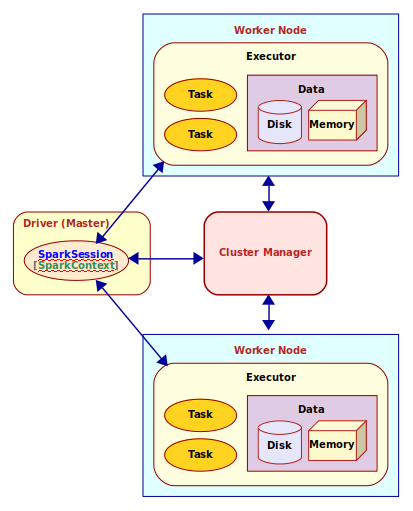
Spark Architecture
The following table summarizes the core components of Apache Spark:
| Component |
Description |
| SparkContext |
Represents a connection to the cluster |
| SparkSession |
Represents a unified higher level abstraction of the cluster |
| Driver |
The process that creates and uses an instance of a SparkSession or a SparkContext |
| Worker Node |
A node in the cluster that executes application code |
| Executor |
A process that is launched for an application on a Worker Node to execute a unit of work (task)
and to store data (in-memory and/or on-disk) |
| Task |
A unit of work that is sent to an Executor |
| Cluster Manager |
A service that is responsible for managing resources on the cluster. It decides which applications can use which
Worker Node and accordingly lauches the Executor process |
Now that we have a basic understanding of the core components of Apache Spark, we can explain some of the variables we
defined in the file /home/polarsparc/Programs/spark-2.4.4/conf/spark-env.sh during the
installation and setup in
Part-1 of this series.
The following are the variables along with their respective description:
| Variable |
Description |
| SPARK_IDENT_STRING |
A string representing a name for this instance of Spark |
| SPARK_DRIVER_MEMORY |
Memory allocated for the Driver process |
| SPARK_EXECUTOR_CORES |
The number of CPU cores for use by the Executor process(es) |
| SPARK_EXECUTOR_MEMORY |
Memory allocated for each Executor process |
| SPARK_LOCAL_IP |
The IP address used by the Driver and Executor to bind to on this node |
| SPARK_LOCAL_DIRS |
The directory to use on this node for storing data |
| SPARK_MASTER_HOST |
The IP address used by the Master to bind to on this node |
| SPARK_WORKER_CORES |
The total number of CPU cores to allow the Worker Node to use on this node |
| SPARK_WORKER_MEMORY |
The total amount of memory to allow the Worker Node to use on this node |
| SPARK_WORKER_DIR |
The temporary directory to use on this node by the Worker Node |
| SPARK_EXECUTOR_INSTANCES |
The number of Worker Nodes to start on this node |
Now that we have a good handle on the basics of Apache Spark, let us get our hands dirty with using Apache Spark.
We will use the Python Spark shell via the Jupyter Notebook to get our hands dirty with Spark Core. So, without much
further ado, lets get started !!!
Open a terminal and change the current working directory to /home/polarsparc/Projects/Python/Notebooks/Spark
Create a sub-directory called data under the current directory.
Next, create a simple text file called Spark.txt under the data
directory with the following contents about Apache Spark (from Wikipedia):
Apache Spark is an open source cluster computing framework originally developed in the AMPLab at University of California,
Berkeley but was later donated to the Apache Software Foundation where it remains today. In contrast to Hadoop's two-stage
disk-based MapReduce paradigm, Spark's multi-stage in-memory primitives provides performance up to 100 times faster for
certain applications. By allowing user programs to load data into a cluster's memory and query it repeatedly, Spark is
well-suited to machine learning algorithms.
Spark requires a cluster manager and a distributed storage system. For cluster management, Spark supports standalone (native
Spark cluster), Hadoop YARN, or Apache Mesos. For distributed storage, Spark can interface with a wide variety, including
Hadoop Distributed File System (HDFS), Cassandra, OpenStack Swift, Amazon S3, Kudu, or a custom solution can be implemented.
Spark also supports a pseudo-distributed local mode, usually used only for development or testing purposes, where distributed
storage is not required and the local file system can be used instead; in such a scenario, Spark is run on a single machine
with one executor per CPU core.
Spark had in excess of 465 contributors in 2014, making it not only the most active project in the Apache Software Foundation
but one of the most active open source big data projects.
In the terminal window, execute the following command to launch the Python Spark shell:
pyspark --master local[1]
This will also launch a new browser window for the Jupyter notebook. The following diagram illustrates the
screenshot of the Jupyter notebook:
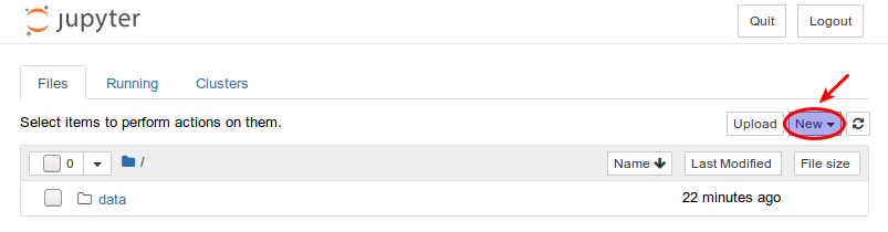
New Notebook
Click on the New drop-down and click on Python3 to create a new
Python notebook. Name the notebook Spark-Notebook-1
The following diagram illustrates the screenshot of the Jupyter notebook:
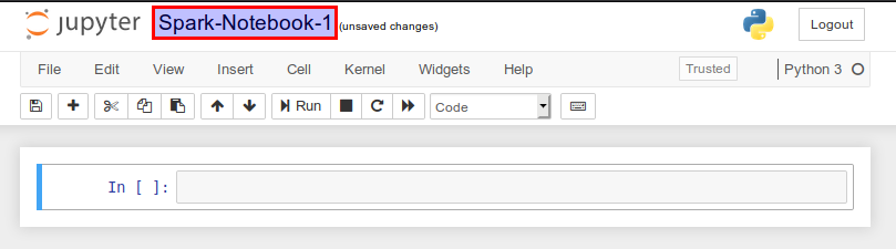
Python3 Notebook
By default, the Python Spark shell in the notebook creates an instance of the SparkContext
called sc. The following diagram illustrates the screenshot of the Jupyter notebook
with the pre-defined SparkContext variable sc:
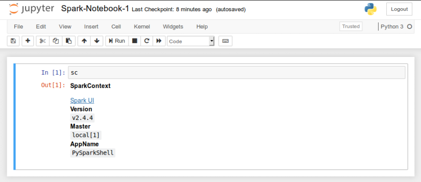
SparkContext in Notebook
In the next cell, type the following command and press ALT + ENTER:
numbers = sc.parallelize(['zero', 'one', 'two', 'three', 'four', 'five', 'six', 'seven', 'eight', 'nine'])
The parallelize() function takes a list as an argument and creates an
RDD. An RDD is the short name for
Resilient Distributed Dataset and is an immutable collection of objects that is partitioned and distributed
across the Worker nodes in a cluster. In other words, an RDD can be operated on in a fault tolerant and parallel
manner across the nodes of a cluster.
In our example above, numbers is an RDD.
The following diagram illustrates the screenshot of the Jupyter notebook with the numbers
RDD:
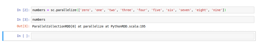
numbers in Notebook
In the next cell, type the following command and press ALT + ENTER:
lines = sc.textFile('./data/Spark.txt')
The textFile() function takes as argument a string that represents the path to a text
file and creates an RDD by loading the contents of the file.
In our example above, lines is an RDD with the contents of the file data/Spark.txt.
The following diagram illustrates the screenshot of the Jupyter notebook with the lines RDD:
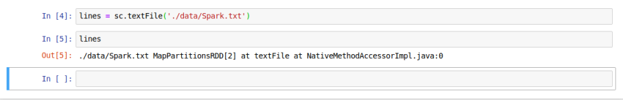
lines in Notebook
In summary, there are two ways to create an RDD from scratch - using the parallelize() function
on a list or using the textFile() on a text file.
In the next cell, type the following command and press ALT + ENTER:
The count() function on an RDD is an action that returns the number of elements in the
specified RDD.
As can be seen from Out[6], we got a result of 10 by executing the count() function on the
numbers RDD.
In the next cell, type the following command and press ALT + ENTER:
As can be seen from Out[7], we got a result of 13 by executing the count() function on the
lines RDD.
The following diagram illustrates the screenshot of the Jupyter notebook with both the counts:
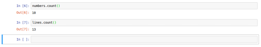
Counts in Notebook
In the next cell, type the following command and press ALT + ENTER:
threes = numbers.filter(lambda s: len(s) == 3)
The filter() function on an RDD is a transformation that returns another RDD that
contains elements from the specified RDD that satisfy the lambda function that was passed to the filter() function.
Tranformation functions are not executed immediately. Instead, they are lazily evaluated; they are evaluated only
when an action function is invoked on them.
In our example above, we create a new RDD called threes by filtering (selecting) all the
words with 3 letters from the numbers RDD.
In the next cell, type the following command and press ALT + ENTER:
sparks = lines.filter(lambda s: 'spark' in s.lower())
In our example above, we create a new RDD called sparks by filtering (selecting) all the
lines that contain the word spark from the lines RDD.
The following diagram illustrates the screenshot of the Jupyter notebook with both the filtered RDDs:
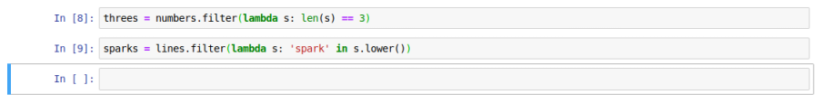
Filters in Notebook
In summary, RDDs support two types of operations - actions and transformations.
Transformations return a new RDD from a specified previous RDD, while Actions compute results that are returned to
the Driver.
In the next cell, type the following command and press ALT + ENTER:
threes.foreach(lambda s: print(s))
The foreach() function on an RDD is an action that applies the specified lambda
function to each element of the specified RDD.
Note that the output is displayed on the terminal window (stdout). As can be seen from the output in the terminal,
we got a result of one, two, and six by executing the foreach() function on the
threes RDD.
In the next cell, type the following command and press ALT + ENTER:
The take() function on an RDD is also an action that returns the specified number
of elements from the specified RDD.
As can be seen from Out[11], we get the 3 lines as a list by executing the
take(3) function on the sparks RDD.
The following diagram illustrates the screenshot of the Jupyter notebook with both the actions:
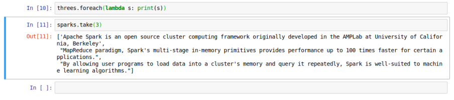
Actions in Notebook
In the next cell, type the following command and press ALT + ENTER:
uppers = threes.map(lambda s : s.upper()
The map() function on an RDD is a transformation that returns another RDD by applying
the specified lambda function to each element of the specified RDD.
In our example above, we create a new RDD called uppers by converting all the words in the
threes RDD to uppercase.
In the next cell, type the following command and press ALT + ENTER:
The collect() function on an RDD is an action that returns all the elements from
the specified RDD. Be very CAUTIOUS of using this function - this function expects all
the objects of the RDD to fit in memory of a single node.
As can be seen from Out[13], we get the 3 words as a list by executing the
collect() function on the uppers RDD.
The following diagram illustrates the screenshot of the Jupyter notebook with the uppers
RDD:
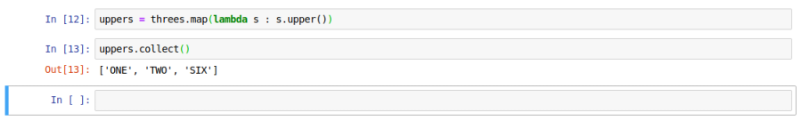
Map in Notebook
In the next cell, type the following command and press ALT + ENTER:
words = sparks.flatMap(lambda s : s.split(' '))
The flatMap() function on an RDD is a transformation that applies the specified lambda
function to each element of the specified RDD and returns a new RDD with the objects from the iterators returned by the
lambda function.
In our example above, we create a new RDD called words by converting all the lines from the
sparks RDD into words.
In the next cell, type the following command and press ALT + ENTER:
The countByValue() function on an RDD is an action that returns the number of times
each element occurs in the specified RDD.
As can be seen from Out[15], we get a dictionary of all the words along with their
respective counts by executing the countByValue() function on the words
RDD.
The following diagram illustrates the screenshot of the Jupyter notebook with the words
RDD:
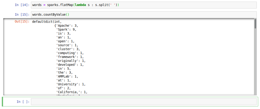
Wordcount in Notebook
To wrap up this part, let us summarize all the transformation and action functions we used thus far in this part.
The following is the summary of the RDD transformation functions we used in this part:
| Tranformation Function |
Description |
| parallelize |
Takes a list of elements as input anc converts it into an RDD |
| textFile |
Takes a string that represents a path to a text file and loads the contents into an RDD |
| filter |
Executed to an existing RDD. Takes a lambda function as input and applies the specified lambda
function to each element of the existing RDD. Returns a new RDD with only those elements that evaluated to true when
the specified lambda function was applied |
| map |
Executed to an existing RDD. Takes a lambda function as input and returns a new RDD by applying
the specified lambda function to each element of the existing RDD |
| flatMap |
Executed to an existing RDD. Takes a lambda function as input and applies the specified lambda
function to each element of the existing RDD. The lambda function returns an iterator for each element. Returns a new
RDD which is a collection of all the elements from all the iterators after flattening them |
The following is the summary of the RDD action functions we used in this part:
| Action Function |
Description |
| count |
Executed to an existing RDD. Returns the number of elements in the specified RDD |
| foreach |
Executed to an existing RDD. Takes a lambda function as input and applies the specified lambda
function to each element of the specified RDD. There is no return value |
| take |
Executed to an existing RDD. Takes a integer as input and returns the specified number of elements
from the specified RDD |
| collect |
Executed to an existing RDD. Returns all the elements from the specified RDD. Use this function
with CAUTION as all the elements from the specified RDD must to fit in memory of this node |
| countByValue |
Executed to an existing RDD. Returns the number of times each element occurs in the specified RDD |