Introduction to Statistics - Part 1
Statistics is the science of collecting, organizing, analyzing, and interpreting numerical
information from data collected from a study (domain of interest).
The collection of all the elements (individuals or objects) from a study is called a Population.
An example would be all the customers of a store from across the country.
A portion or subset of elements from the Population is called a
Sample. An example for a Sample would
be a selection of 100 customers of a store from a particular location.
There are two types of statistics - Descriptive and Inferential.
| Name |
Description |
| Descriptive Statistics |
focuses on organizing, summarizing, and displaying data using tables and graphs |
| Inferential Statistics |
focuses on analyzing data about the Sample to arrive at a
conclusion about the Population |
A Random Sample is a Sample in which each element from the
Population has an equal chance of being selected. An example for a Random
Sample would be a random selection of 100 customers of a store from across the country.
A Variable is a characteristic of the elements in a Sample
that can be observed (or measured). An example would be the annual income of a customer.
A value of a Variable is referred to as an Observation
(or Measurement).
A collection of Observations (or Measurements) is referred to as a
Data Set.
There are two types of data Variables - Quantitative and
Qualitative.
| Name |
Description |
| Quantitative |
data variables can be measured numerically. An example would be the monthly expense
for a customer |
| Qualitative |
data variables are non-numerically and can only be categorized (or grouped) and counted. An
example would be the brand of car driven by a customer |
Quantitative data variables can further be divided into two types - Discrete
and Continuous.
| Name |
Description |
| Discrete |
data variables are countable. An example would be the number of credit cards a customer has |
| Continuous |
data variables have a numerical value over a certain interval range. An example would be the
monthly account balance of a customer |
There are four levels of Measurements - Nominal,
Ordinal, Interval, and Ratio.
| Name |
Description |
| Nominal |
measurements involve names or labels (not numerical). Can only be counted. An example would be
the credit card preference (amex, mastercard, visa) of a customer |
| Ordinal |
measurements involve names or labels (not numerical). Can be counted or arranged in an order.
An example would be the customer service rating (good, average, bad) from a customer |
| Interval |
measurements involve numerical values. Can be arranged in an order. Basic arithmetic operations
such as additions or subtractions possible (and make sense). Do not have a true zero value. An example would be
the room temperature |
| Ratio |
measurements involve numerical values. Basic arithmetic operations such as additions, subtractions
and divisions possible (and make sense). Have a true zero value to indicate absence of a value. An example would be the
monthly deposits from a customer |
Basic Data Visualization Using Graphs
Consider the following raw data on the type of credit card used from a random sample of 10 customers:
{ Visa, Discover, Visa, Amex, MasterCard, Visa, MasterCard, Amex, Visa, MasterCard }
The above qualitative raw data set can be organized and presented in a tablular form using
Frequency Distribution or using Relative Frequency
A Frequency Distribution lists all the unique types (or categories)
along with their occurrence count.
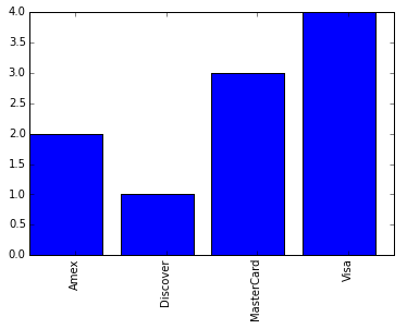
The following is the Frequency Distribution table of the above raw data set:
| Credit Card Type |
Frequency |
| Amex |
2 |
| Discover |
1 |
| MasterCard |
3 |
| Visa |
4 |
A Frequency Distribution for a qualitative data set is graphically represented using a
Bar Chart with the x-axis representing the various categories and the y-axis representing
the frequencies.
The following is the Bar Chart for the above Frequency Distribution:
Bar Chart
A Relative Frequency for a type (or category) is computed by dividing the
Frequency Distribution of the type (or category) by the sum of all frequencies.
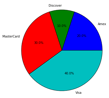
The following is the Relative Frequency table of the above raw data set:
| Credit Card Type |
Relative Frequency |
| Amex |
2/10 = 0.2 |
| Discover |
1/10 = 0.0 |
| MasterCard |
3/10 = 0.3 |
| Visa |
4/10 = 0.4 |
A Relative Frequency is graphically represented using a Pie Chart
with the segments representing the various categories and the angles representing the relative frequency in percentage.
To convert a Relative Frequency to a percentage, just multiple the
Relative Frequency value with 100. For example, a Relative Frequency
of 0.3 = 0.3 * 100% = 30%.
The following is the Pie Chart for the above Relative Frequency:
Pie Chart
Consider the following raw data on the number of credit card transactions per month from a random sample of 20 customers:
{ 11, 27, 9, 13, 26, 15, 24, 38, 17, 10, 34, 13, 41, 28, 33, 14, 31, 8, 44, 7 }
The above quantitative raw data set can be organized and presented in a tablular form using
Frequency Distribution (or Frequency Table).
For a quantitative raw data set with large number of elements, it is better to organize them into a handful of intervals
(or classes) and count the number of data elements that fall into each of the intervals (or classes).
The following are the steps to create a Frequency Distribution table for the
quantitative raw data set indicated above:
-
Decide on the number of classes. It is typically between 5 and 20 depending on the number
of observations in the data set.
As a general rule of thumb, use the Sturge's formula as follows:
c = 1 + 3.3 * log(n)
where: c = no. of classes, n = no. of observations in the data set
For our data set, we choose c = 6.
-
Determine the class width. The class width is defined using the following formula:
class width = ceiling of [(largest value - smallest value) / no. of classes]
For our data set, largest value = 44, smallest value = 7
class width = ceiling of [(44 - 7) / 6 = 6.1] = 7
-
Determine the class limits. The lower limit of the first class is the smallest value in
the data set. The upper limit of the first class is the lower limit plus the class width minus 1. The lower limit of the
next class is the lower limit of the previous class plus the class width.
For our data set, the smallest value = 7. Hence, the lower limit of the first class is 7. The upper limit is lower limit
which is 7 plus the class width which is 7 minus 1 equal to 13. The lower limit of the next class is the lower limit of
the previous class which is 7 plus the class width which is 7 equals 14.
Following the above steps, the given quantitative raw data set can be organized and presented in a tablular form using the
Frequency Distribution table as shown below:
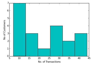
| Class Range (No. of Transactions) |
Frequency (No. of Customers) |
| 7-13 |
7 |
| 14-20 |
3 |
| 21-27 |
1 |
| 28-34 |
4 |
| 35-41 |
2 |
| 42-48 |
3 |
A Frequency Distribution table for quantitative data set is graphically represented using an
Histogram with the x-axis representing the class intervals and the y-axis representing the
frequencies.
The following is the Histogram for the above Class Frequency table:
Histogram
!!! ATTENTION !!!
Statistics is a tool to analyze a sample data set to obtain an estimate about the population. It would be nearly impossible to analyze the entire population data set in a timely manner to arrive at a conclusion.
Measures of Central Tendency
A measure of central tendency gives us the center of frequency distribution for a given data set.
There are three types of measures of central tendency - Mean, Median,
and Mode.
The Mean (also referred to as Arithmetic Mean) is computed by
dividing the sum of all the values in the data set by the number of values in the data set.
Mean = Sum of all the values in the data set / Number of values in the data set
The Mean of a population is represented using the symbol \(\mu\),
while the Mean of a sample is represented using the symbol \(\bar{x}\).
Mathematically,
For Population: \(\mu = \)\(\Large{\frac{\Sigma{X_i}}{N}}\), where i = 1 to N
and
For Sample: \(\bar{x} = \)\(\Large{\frac{\Sigma{x_i}}{n}}\), where i = 1 to n
| Example-1 |
The following are the annual salaries (in thousands) of ten employees of a company:
{ 45, 33, 56, 28, 61, 26, 48, 65, 36, 22 }. Find the mean salary of the employees.
|
|
There are 10 values in the data set. n = 10.
\(\sum_{i = 1}^{10}{x_i}\) = 45 + 33 + 56 + 28 + 61 + 26 + 48 + 65 + 36 + 22 = 420.
The sample mean \(\bar{x} = \)\(\Large{\frac{\sum_{i = 1}^{10}{x_i}}{n}}\) = 420 / 10 = 42.
The mean salary of the employees is 42.
|
When the data set is in the form of a frequency distribution, the Mean is computed as follows:
For Population: \(\mu = \)\(\Large{\frac{\Sigma{X_i * f_i}}{\Sigma{f_i}}}\), where i = 1 to N
and
For Sample: \(\bar{x} = \)\(\Large{\frac{\Sigma{x_i * f_i}}{\Sigma{f_i}}}\), where i = 1 to n
| Example-2 |
The following are the frequency distributions of annual salaries (in thousands) of twenty employees of a company:
{ (45, 3), (33, 4), (56, 2), (28, 5), (61, 2), (22, 4) }. Find the mean salary of the employees.
|
|
Since this is a frequency distribution, we need to use the formula:
\(\bar{x} = \)\(\Large{\frac{\Sigma{x_i * f_i}}{\Sigma{f_i}}}\), where i = 1 to n
\(\Sigma{x_i * f_i}\) (where i = 1 to 10) = (45 * 3) + (33 * 4) + (56 * 2) + (28 * 5) + (61 * 2) + (22 * 4) = 729.
\(\Sigma{f_i}\) (where i = 1 to 10) = 3 + 4 + 2 + 5 + 2 + 4 = 20.
\(\bar{x} = \)\(\Large{\frac{\Sigma{x_i * f_i}}{\Sigma{f_i}}}\) (where i = 1 to 10) = 729 / 20 = 36.45.
The mean salary of the employees is 36.45.
|
!!! CAUTION !!!
Mean is sensitive to outliers or extreme data values.
The Median is the middle value in an ordered data set.
To find the median for a given data set:
-
Order the data set in an ascending order
-
If there are odd number of observations in the data set, the Median is the
value in the middle of the ordered data set
-
If there are even number of observations in the data set, the Median is the
average of the middle two values of the ordered data set
| Example-3 |
The following are the annual salaries (in thousands) of nine employees of a company:
{ 45, 33, 56, 28, 61, 26, 48, 65, 36 }. Find the median salary of the employees.
|
|
Arranging the given salaries in an ascending order, we get the ordered data set { 26, 28, 33, 36, 45, 48, 56, 61, 65 }.
Since we have an odd number of values in the ordered data set, the Median is the middle value,
which is the fifth element in the ordered data set of 45.
The median salary of the employees is 45.
|
Lets look at another example with even number of values in the data set.
| Example-4 |
The following are the annual salaries (in thousands) of ten employees of a company:
{ 45, 33, 56, 28, 61, 26, 48, 65, 36, 22 }. Find the median salary of the employees.
|
|
Arranging the given salaries in an ascending order, we get the ordered data set { 22, 26, 28, 33, 36, 45, 48, 56, 61, 65 }.
Since we have an even number of values in the ordered data set, the Median is the average of the
middle two value, which are the averages of fifth and sixth element in the ordered data set.
(36 + 45) / 2 = 40.5.
The median salary of the employees is 40.5.
|
The Mode is the value in the given data set that occurs most frequently.
| Example-5 |
The following are the annual salaries (in thousands) of ten employees of a company:
{ 45, 33, 56, 28, 61, 28, 48, 65, 36, 28 }. Find the mode for the given data set.
|
|
For the given data set, the value 28 occurs most frequently - it occurs 3 times.
Hence, the mode is 28.
|
It is possible that for a given data set thete is no Mode. This happens when there is
no data value that occurs the most.
| Example-6 |
The following are the annual salaries (in thousands) of ten employees of a company:
{ 45, 33, 56, 28, 61, 26, 48, 65, 36, 22 }. Find the mode for the given data set.
|
|
For the given data set, all the values occur only once.
Hence there is *NO* mode.
|
!!! ATTENTION !!!
The Mean is the most commonly used measure for central tendency.
Measures of Dispersion (or Variation)
As indicated earlier, the measures of central tendency provide us the center of the frequency distribution for a given data
set. In fact, two data sets can have the same mean, but may be differently spread.
Lets look at example to illustrate the point. Look at the salaries (in thousands) of employees from two companies.
Company A: { 42, 38, 34, 45, 36 }, Mean: 39
Company B: { 18, 77, 53, 12, 35 }, Mean: 39
Both the data sets have the same mean, but the values in Company A are more closely clustered, while the values in Company
B are spread far apart.
The measures of dispersion allow us to learn about the spread of values for a given data set around the mean.
There are two types of measures of dispersion - Variance and
Standard Deviation.
The Variance is computed as the average of the squared deviations for a given data set.
To find the variance for a given data set:
-
Compute the mean (\(\mu\) or \(\bar{x}\)) for the given data set
-
Compute the deviation for each value in the given data set.
If \(x_i\) is the ith value of the data set, then:
For Population: deviation = \(X_i - \mu\)
For Sample: deviation = \(x_i - \bar{x}\)
-
Compute the square of the deviation for each value in the given data set.
For Population: \({deviation_i}^2 = (X_i - \mu)^2\)
For Sample: \({deviation_i}^2 = (x_i - \bar{x})^2\)
-
The Variance of a population is denoted using the symbol \(\sigma^2\),
while the Variance of a sample is denoted using the symbol \(s^2\).
To find the variance, sum all the squares of the deviation for each value in the given data set and divide by the number
of values in the given data set.
For Population: \(\sigma^2\) = \(\Large{\frac{\Sigma{deviation_i^2}}{N}}\), where i = 1 to N
For Sample: \(s^2\) = \(\Large{\frac{\Sigma{deviation_i^2}}{(n - 1)}}\), where i = 1 to n
For a sample, we divide by (n-1) so that we obtain a better estimate of the variance. Various tests have proved that the
estimates obtained by diving by n are smaller than the true variance.
| Example-7 |
The following are the annual salaries (in thousands) of ten employees of a company:
{ 45, 33, 56, 28, 61, 26, 48, 65, 36, 22 }. Calculate the variance for the given data set.
|
|
The number of values in the sample data set n = 10.
The mean \(\bar{x} = \)\(\Large{\frac{\Sigma{x_i}}{n}}\) (where i = 1 to 10) = 420 / 10 = 42.
Computing the deviation of the sample data set: { (45 - 42), (33 - 42), (56 - 42), (28 - 42), (61 - 42),
(26 - 42), (48 - 42), (65 - 42), (36 - 42), (22 - 42) }.
The deviation of the sample data set is: { 3, -9, 14, -14, 19, -16, 6, 23, -6, -20 }.
The squared deviation of the sample data set is: { 9, 81, 196, 196, 361, 256, 36, 529, 36, 400 }.
The variance of the sample \(s^2\) = \(\Large{\frac{\Sigma{deviation_i^2}}{(n - 1)}}\) = (9+81+196+196+361+256+36+529+36+400)/(10-1) = 233.33.
The variance for the given sample data set is 233.33.
|
The Standard Deviation is computed by taking the square root of the
Variance for a given data set.
The Standard Deviation of a population is denoted using the symbol \(\sigma\),
while the Standard Deviation of a sample is denoted using the symbol s.
| Example-8 |
The following are the annual salaries (in thousands) of five employees of a company:
{ 42, 38, 34, 45, 36 }. Calculate the standard deviation for the given data set.
|
|
The number of values in the sample data set n = 5.
The mean \(\bar{x} = \)\(\Large{\frac{\Sigma{x_i}}{n}}\) (where i = 1 to 5) = 195 / 5 = 39.
Computing the deviation of the sample data set: { (42 - 39), (38 - 39), (34 - 39), (45 - 39), (36 - 39) }.
The deviation of the sample data set is: { 3, -1, -5, 6, -3 }.
The squared deviation of the sample data set is: { 9, 1, 25, 36, 9 }.
The variance of the sample \(s^2\) = \(\Large{\frac{\Sigma{deviation_i^2}}{(n - 1)}}\) = (9+1+25+36+9)/(5-1) = 20.
The variance for the given sample data set \(s^2\) = 20.
The standard deviation for the given sample data set s = \(\sqrt{s^2}\) = \(\sqrt{20}\) = 4.47.
|
Let us look at another example that has the same mean as in Example-8 but a very different variation.
| Example-9 |
The following are the annual salaries (in thousands) of five employees of a company:
{ 18, 77, 53, 12, 35 }. Calculate the standard deviation for the given data set.
|
|
The number of values in the sample data set n = 5.
The mean \(\bar{x} = \)\(\Large{\frac{\Sigma{x_i}}{n}}\) (where i = 1 to 5) = 195 / 5 = 39.
Computing the deviation of the sample data set: { (18 - 39), (77 - 39), (53 - 39), (12 - 39), (35 - 39) }.
The deviation of the sample data set is: { -21, 38, 14, -27, -4 }.
The squared deviation of the sample data set is: { 441, 1444, 196, 729, 16 }.
The variance of the sample \(s^2\) = \(\Large{\frac{\Sigma{deviation_i^2}}{(n - 1)}}\) = (441+1444+196+729+16)/(5-1) = 706.5.
The variance for the given sample data set \(s^2\) = 706.5.
The standard deviation for the given sample data set s = \(\sqrt{s^2}\) = \(\sqrt{706.5}\) = 26.58.
|
!!! ATTENTION !!!
The Standard Deviation is the most commonly used measure for dispersion (or variation).
Range, Percentile, and Quartile
A Range is simplest measure of dispersion and is computed by finding the difference between
the largest value and the smallest value in a data distribution.
The Percentile divides the data distribution into 100 equal ranges. The Pth percentile of a
distribution is a value such that P% of the data fall at or below it.
A Quartile measures the relative position of a data distribution by dividing the distribution
into 4 equal ranges. The first quartile is the 25th percentile, the second quartile is the median, and the third quartile is
the 75th percentile.
To find the quartile for a given data set:
-
Arrange the given data set from the smallest to the largest (ascending order)
-
Find the median of the sorted data set. That is the second quartile (Q2) or the 50th percentile
-
Find the median of the lower half of the sorted data set (below Q2). That is the first quartile (Q1) or the 25th percentile
-
Find the median of the upper half of the sorted data set (above Q2). That is the third quartile (Q3) or the 75th percentile
Given the data set { 45, 33, 56, 28, 61, 26, 48, 36, 22 }, the following is the Box-and-Whisker Plot
(or Box Plot) for the data set:
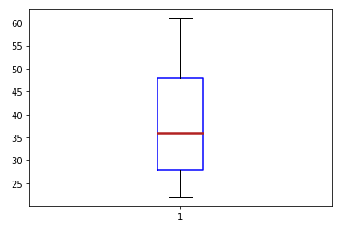
Box-and-Whisker Plot
The Box-and-whisker plots (or Box plots) provide a visual display of the spread of data about the median of the given data
set.
| Example-10 |
The following are the annual salaries (in thousands) of 10 employees of a company:
{ 45, 33, 56, 28, 61, 26, 48, 36, 22, 65 }. Find the Quartile values for the given data set.
|
|
First step is to arrange the data set in an ascending order: { 22, 26, 28, 33, 36, 45, 48, 56, 61, 65 }.
The second step is to find the median of the data set: Q2 = (36 + 45)/2 = 40.5.
The third step is to find the median of lower half of Q2: Q1 = 28.
The final step is to find the median o upper half of Q2: Q3 = 56.
Hence, the Quartile values are: Q1 = 28, Q2 = 40.5, and Q3 = 56.
|