Machine Learning - Data Preparation

Machine Learning - Data Preparation - Part 2

Bhaskar S

05/22/2022

Overview

In Part 1 of this series, we used the the City of Ames, Iowa Housing Prices data set to perform the various tasks related to the Exploratory Data Analysis (EDA) to gather some insights about the loaded data set. In this part, we will first explain the approach to handling missing values that is related to Feature Engineering, followed by hands-on demo in Python.

Feature Engineering - Missing Values

For crafting a good machine learning model, the model algorithm requires that all feature values (from the training data set as well as the test data set) be numerical values and that there are no missing data values.

If the number of samples (rows) with missing data values (from the data set) is very small, say less than 1%, then one can drop the rows (with the missing data) from the data set without impacting the model creation and evaluation. However, if the number of samples (rows) with missing data values is large (say > 5%), then one cannot drop the rows and instead perform data Imputation.

Imputation is the process of identifying and replacing missing values for each of the features from a data set before it is used for training and testing a machine learning model.

The following are some of the commonly used strategies for imputing missing values:

Mean Imputation - If a numerical feature variable (a column in the dataframe) with missing values is normally distributed, then the missing values can be replaced with the mean of that feature variable
Median Imputation - If a numerical feature variable (a column in the dataframe) with missing values is either left or right skewed distribution, then the missing values can be replaced with the median of that feature variable
Most Frequent Imputation - Also known as Mode Imputation, it is typically applied to categorical feature variables (with string or numbers) and replaces the missing values with the most frequent value from that feature variable
Constant Value Imputation - For a numerical feature variable (a column in the dataframe) with missing values, it replaces the missing values with an arbitrary constant number such as a -1, or a 0, etc. For a categorical feature variable with missing values, it replaces the missing values with an arbitrary constant string such as 'None', or 'Missing', etc
Random Value Imputation - It is applicable to both the categorical and numerical feature variables (a column in the dataframe) and it replaces each missing value with a random sample from the set of unique values of that feature variable

Hands-On Data Imputation

The first step is to import all the necessary Python modules such as, matplotlib, pandas, and seaborn as shown below:

import pandas as pd
import matplotlib.pyplot as plt
import seaborn as sns

The next step is to load the housing price dataset into a pandas dataframe as shown below:

url = './data/ames.csv'
ames_df = pd.read_csv(url)

The next step is to drop some of the features that add no value, or have large number (above 80%) of missing values, or have low correlation to the target feature (SalePrice) from the housing price dataset as shown below:

home_price_df = ames_df.drop(['Order', 'PID', 'Pool.QC', 'Misc.Feature', 'Alley', 'Fence', 'MS.SubClass', 'Lot.Frontage', 'Lot.Area', 'Overall.Cond', 'BsmtFin.SF.1', 'BsmtFin.SF.2', 'Bsmt.Unf.SF', 'X2nd.Flr.SF', 'Low.Qual.Fin.SF', 'Bsmt.Full.Bath', 'Bsmt.Half.Bath', 'Half.Bath', 'Bedroom.AbvGr', 'Kitchen.AbvGr', 'Fireplaces', 'Wood.Deck.SF', 'Open.Porch.SF', 'Enclosed.Porch', 'X3Ssn.Porch', 'Screen.Porch', 'Pool.Area', 'Misc.Val', 'Mo.Sold', 'Yr.Sold'], axis=1)

The next step is to display the shape (rows and columns) of the housing price dataset as shown below:

home_price_df.shape

The following illustration shows the shape of the housing price dataset:

Figure.1

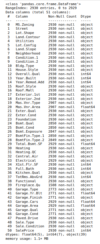
The next step is to display information about the housing price dataframe, such as index and column types, missing (null) values, memory usage, etc., as shown below:

home_price_df.info()

The following illustration displays the information about the housing price dataframe:

Figure.2

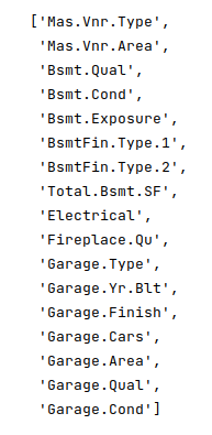
The next step is to display the feature names from the housing price dataframe that have missing (nan) values as shown below:

features_na = [feature for feature in ames_df.columns if ames_df[feature].isnull().sum() > 0]
features_na

The following illustration displays the list of all the feature names from the housing price dataframe with missing values:

Figure.3

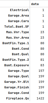
The next step is to display the features and the count of their missing values from the housing price dataframe as shown below:

home_price_df[features_na].isnull().sum().sort_values()

The following illustration displays the list of the feature names along with the count of their missing value from the housing price dataframe:

Figure.4

The next step is to display the rows corresponding to the features Electrical, Garage.Area, Garage.Cars, and Total.Bsmt.SF with one missing value from the housing price dataframe as shown below:

home_price_df[home_price_df['Garage.Cars'].isnull() | home_price_df['Garage.Area'].isnull() | home_price_df['Total.Bsmt.SF'].isnull() | home_price_df['Electrical'].isnull()]

The following illustration displays the rows with one missing value from the housing price dataframe:

Figure.5

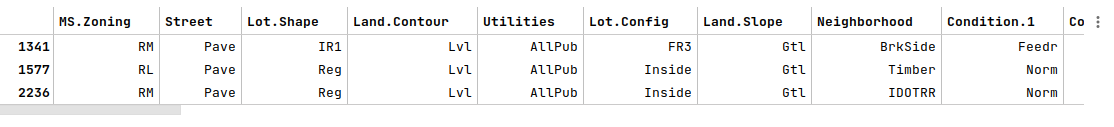
Given that it is only 3 of the 2930 rows from the housing price data set with one missing value, it is okay to drop these rows.

The next step is drop the 3 rows with a missing value from the housing price dataframe as shown below:

one_na_index = home_price_df[home_price_df['Garage.Cars'].isnull() | home_price_df['Garage.Area'].isnull() | home_price_df['Total.Bsmt.SF'].isnull() | home_price_df['Electrical'].isnull()].index
home_price_df = home_price_df.drop(one_na_index, axis=0)

The next step is to re-evaluate the features with missing values and display the count of their missing values from the housing price dataframe as shown below:

features_na = [feature for feature in home_price_df.columns if home_price_df[feature].isnull().sum() > 0]
home_price_df[features_na].isnull().sum().sort_values()

The following illustration displays the list of the feature names along with the count of their missing value from the housing price dataframe:

Figure.6

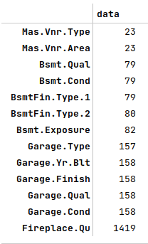
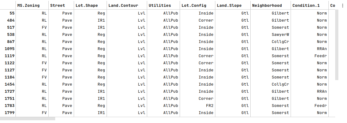
The next step is to display the rows corresponding to the features Mas.Vnr.Type and Mas.Vnr.Area with 23 missing values from the housing price dataframe as shown below:

home_price_df[home_price_df['Mas.Vnr.Type'].isnull() | home_price_df['Mas.Vnr.Area'].isnull()]

The following illustration displays the rows with 23 missing values from the housing price dataframe:

Figure.7

Looking at the data dictionary of the Ames Housing Price data set, the acceptable value for Mas.Vnr.Type is 'None' and the for Mas.Vnr.Area would be 0.

The next step is to replace the missing values for Mas.Vnr.Type and Mas.Vnr.Area from the housing price dataframe as shown below:

home_price_df['Mas.Vnr.Type'].fillna('None', inplace=True)
home_price_df['Mas.Vnr.Area'].fillna(0, inplace=True)

The next step is to once again to re-evaluate the features with missing values and display the count of their missing values from the housing price dataframe as shown below:

features_na = [feature for feature in home_price_df.columns if home_price_df[feature].isnull().sum() > 0]
home_price_df[features_na].isnull().sum().sort_values()

The following illustration displays the list of the feature names along with the count of their missing value from the housing price dataframe:

Figure.8

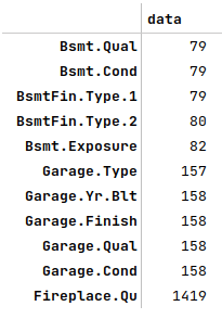
The next step is to display the rows corresponding to the features Bsmt.Qual, Bsmt.Cond, BsmtFin.Type.1, BsmtFin.Type.2, and Bsmt.Exposure with about 80+ missing values from the housing price dataframe as shown below:

home_price_df[home_price_df['Bsmt.Qual'].isnull() | home_price_df['Bsmt.Cond'].isnull() | home_price_df['BsmtFin.Type.1'].isnull() | home_price_df['BsmtFin.Type.2'].isnull() | home_price_df['Bsmt.Exposure'].isnull()]

The following illustration displays the rows with about 80+ missing values from the housing price dataframe:

Figure.9

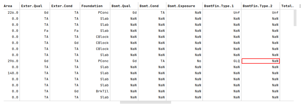
The row at index 444 has a value for BsmtFin.Type.1 but not for BsmtFin.Type.2. Looking at the data dictionary for the Ames Housing Price data set, we can infer we can use of 'GLQ' (for good living quarters).

The next step is to replace the missing value for BsmtFin.Type.2 at index 444 from the housing price dataframe as shown below:

home_price_df.loc[444, 'BsmtFin.Type.2'] = 'GLQ'

The next step is to replace the missing values for Bsmt.Qual, Bsmt.Cond, BsmtFin.Type.1, BsmtFin.Type.2, and Bsmt.Exposure from the housing price dataframe as shown below:

home_price_df['Bsmt.Qual'].fillna('NA', inplace=True)
home_price_df['Bsmt.Cond'].fillna('NA', inplace=True)
home_price_df['BsmtFin.Type.1'].fillna('NA', inplace=True)
home_price_df['BsmtFin.Type.2'].fillna('NA', inplace=True)
home_price_df['Bsmt.Exposure'].fillna('NA', inplace=True)

The next step is to once again to re-evaluate the features with missing values and display the count of their missing values from the housing price dataframe as shown below:

features_na = [feature for feature in home_price_df.columns if home_price_df[feature].isnull().sum() > 0]
home_price_df[features_na].isnull().sum().sort_values()

The following illustration displays the list of the feature names along with the count of their missing value from the housing price dataframe:

Figure.10

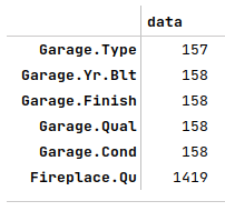
The next step is to display the rows corresponding to the features Garage.Type, Garage.Yr.Blt, Garage.Finish, Garage.Qual, and Garage.Cond with about 158 missing values from the housing price dataframe as shown below:

home_price_df[home_price_df['Garage.Type'].isnull() | home_price_df['Garage.Yr.Blt'].isnull() | home_price_df['Garage.Finish'].isnull() | home_price_df['Garage.Qual'].isnull() | home_price_df['Garage.Cond'].isnull()]

The following illustration displays the rows with about 158 missing values from the housing price dataframe:

Figure.11

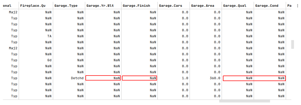
The row at index 1356 has a value for Garage.Type but not for Garage.Yr.Blt, Garage.Finish, Garage.Qual, and Garage.Cond.

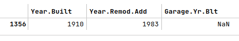
The missing value for Garage.Yr.Blt can be determined by looking at the values for other features such as Year.Built and Year.Remod.Add.

The next step is to display the values corresponding to the features Year.Built, Year.Remod.Add, and Garage.Yr.Blt for the row at index 1356 from the housing price dataframe as shown below:

home_price_df.loc[[1356], ['Year.Built', 'Year.Remod.Add', 'Garage.Yr.Blt']]

The following illustration displays the values corresponding to the features Year.Built, Year.Remod.Add, and Garage.Yr.Blt at index 1356 from the housing price dataframe:

Figure.12

The next step is to display a count plot for Garage.Finish to determine the most frequent value using the housing price data set as shown below:

sns.countplot(x='Garage.Finish', data=home_price_df)
plt.show()

The following illustration shows the count plot for Garage.Finish using the housing price data set:

Figure.13

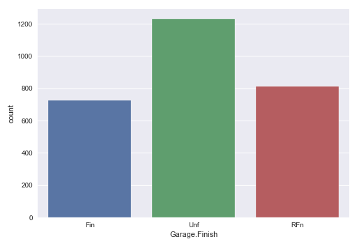
Notice that the value of 'Unf' is the most frequent value for Garage.Finish.

The next step is to display a count plot for Garage.Qual to determine the most frequent value using the housing price data set as shown below:

sns.countplot(x='Garage.Qual', data=home_price_df)
plt.show()

The following illustration shows the count plot for Garage.Qual using the housing price data set:

Figure.14

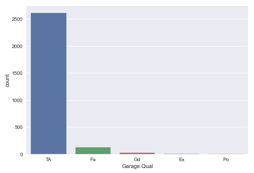
Notice that the value of 'TA' is the most frequent value for Garage.Qual.

The next step is to display a count plot for Garage.Cond to determine the most frequent value using the housing price data set as shown below:

sns.countplot(x='Garage.Cond', data=home_price_df)
plt.show()

The following illustration shows the count plot for Garage.Cond using the housing price data set:

Figure.15

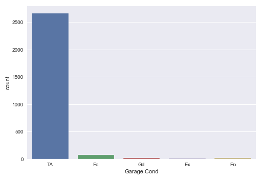
Notice that the value of 'TA' is the most frequent value for Garage.Cond.

The next step is to replace the missing values for Garage.Yr.Blt, Garage.Type, Garage.Finish, Garage.Qual, and Garage.Cond at index 1356 (from the information gathered above) in the housing price dataframe as shown below:

home_price_df.loc[1356, 'Garage.Yr.Blt'] = home_price_df.loc[1356, 'Year.Built']
home_price_df.loc[1356, 'Garage.Finish'] = 'Unf'
home_price_df.loc[1356, 'Garage.Qual'] = 'TA'
home_price_df.loc[1356, 'Garage.Cond'] = 'TA'

The next step is to replace the missing values for Garage.Yr.Blt, Garage.Type, Garage.Finish, Garage.Qual, and Garage.Cond from the housing price dataframe as shown below:

home_price_df['Garage.Yr.Blt'].fillna(0, inplace=True)
home_price_df['Garage.Type'].fillna('NA', inplace=True)
home_price_df['Garage.Finish'].fillna('NA', inplace=True)
home_price_df['Garage.Qual'].fillna('NA', inplace=True)
home_price_df['Garage.Cond'].fillna('NA', inplace=True)

The next step is to replace the missing values for Fireplace.Qu from the housing price dataframe as shown below:

home_price_df['Fireplace.Qu'].fillna('NA', inplace=True)

The next step is to display the count for all the missing values from the housing price dataframe as shown below:

home_price_df.isnull().sum()

The following illustration shows the count for all the missing values from the housing price data set:

Figure.16

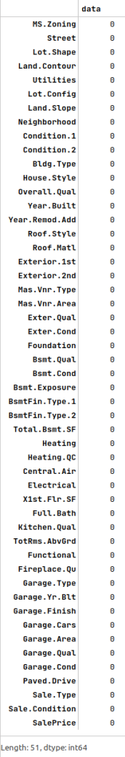
At this point we have no missing values in the housing price data set.

Hands-on Demo

The following is the link to the Jupyter Notebooks that provides an hands-on demo for this article:

Data Preparation - Part 2

References

Machine Learning - Data Preparation - Part 1