Figure.1
| PolarSPARC |
Introduction to Deep Learning - Part 2
| Bhaskar S | 05/29/2023 |
Introduction
In Introduction to Deep Learning - Part 1 of this series, we introduced the concept of a perceptron, followed by the concept of a neural network, and finally the concept of an activation function.
In this article, we will continue the journey, diving deeper into the core of neural network to get a better intuition of its inner workings.
Feed Forward Network
From the previous article, we know that a neural network is an artificial equivalent of a human brain, with a complex network perceptrons, arranged in layers.
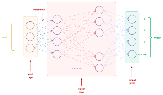
The following illustration depicts the structure of an artificial neural network:
With this type of neural network structure, the input data moves from the input layer to one or more hidden layer(s), before coming off the output layer as a final prediction. In other words, the input flows forward without any feedback cycle between the nodes of the neural network.
At this point, one may have a question - how does one begin to train a neural network model to be effective at future predictions ???
For that one needs a large amount of training data with the actual predictions tagged.
The following are the high-level steps to train a neural network model:
Initialize the weight and the bias (parameter ) for each of the connections between the nodes of the neural network to some random value
Feed each sample from the training dataset to the neural network model and measure the error made by the model in making the prediction versus the actual prediction
Compute the average prediction error for the entire training dataset
If the average prediction error is above some threshold value, adjust the weights and the biases of the neural network so as to MINIMIZE the prediction error of the model and repeat the training process again
What we have outlined above are a very high-level set of steps to train a neural network model. In the following paragraphs we will zoom in to the details.
Loss Function
As a neural network makes a prediction for a given input, we need a way to measure the deviation (or the prediction error) from the actual target prediction. The numerical value of the deviation (or the prediction error) is often referred to as a Loss or a Cost.
The function used to compute the prediction error is often referred to as the Loss Function or a Cost Function.
There are several types of loss functions to choose from based on the type of the problem the neural network model is trying to solve for, such as, a classification or a regression problem.
For this article, we will use the Mean Sqaured Error as the loss function $L(x, W, b)$, which is defined as follows:
$L(x, W, b) = (\sigma(x, W, b) - y)^2$
where, $x$ is the input, $W$ is the weights, $b$ is the biases, $\sigma$ is the activation function with its output as the predicted value, and $y$ is the actual target prediction value.
Gradient Descent
As indicated in the high-level steps above, the main idea is to tune the neural network model by MINIMIZING the loss of the model. This is where the concept of Gradient Descent comes into play.
Now, the question one would have is - how does one minimize the error from a function ???
Well, the answer to that question would be - Derivatives from Calculus to the rescue !!!
The MINIMUM of a function occurs when the derivative of that function is ZERO.
Let us look at an example to get a better understanding of this concept.
Let $y$ be a function of $x$ as defined below:
$y = x^2 - 3.x + 1$
Then, the derivative of the function $y$ with respect to $x$ is as follows:
$\Large{\frac{dy}{dx}}\normalsize{= 2.x - 3}$
The following illustration shows the plots for $y$ and its derivative $\Large{\frac{dy}{dx}}$:
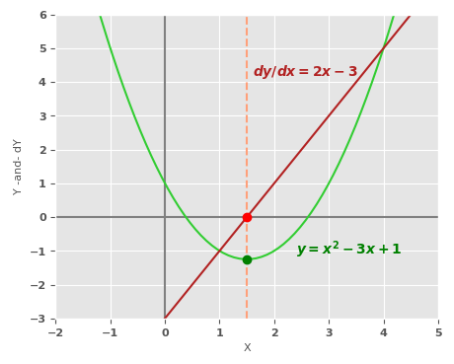
As is evident from the plot in Figure.2 above, the function minimum (green dot) occurs when its derivative $\Large{\frac{dy}{dx}}$ is zero (red dot).
It is easy for humans to look at the plot in Figure.2 above and deduce where the the function minimum occurs. How about computers ???
This is where the algorithm for gradient descent comes in handy.
The following are the high-level steps for gradient descent:
Initialize the Maximum Number of Iterations (also called Epochs) and the Learning Rate (denoted using the symbol $\eta$)
Initialize the minimum value ($min$) of a function to a random value
For each iteration upto the maximum number of iterations (epochs), perform the following steps:
The final minimum value ($min$) will be an approximation for the minimum of the function
The following illustration shows the points traversed by the gradient descent algorithm before the final stop (function minimum) for two cases - one from the left and one from the right:
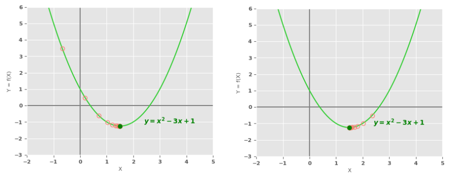
Note that the final function minimum will be a close approximation, but NOT an exact value.
The gradient descent algorithm is akin to the approach taken by a person, who wants to reach the the valley at the bottom of a mountain as shown in the illustration below:
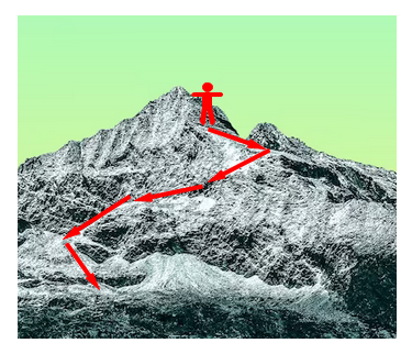
The person moves forward at each step when the slope is downward (hence descent).
The Learning Rate controls how quickly the algorithm will learn about the function minimum. If the value is SMALL, the learning will take a longer time and on the other hand, if the value is LARGE, the learning may result in a sub-optimal solution (wrong minimum). One needs to tune the learning rate for an optimal value. The value of 0.01 is typically a good start.
The plot of the function $y = x^2 - 3.x + 1$ as shown in the Figure.2 above was a simple polynomial of $2^{nd}$ degree and had a single minimum, which was easy to identify.
Now, let us look at a more complex polynomial function of the $4^{th}$ degree. The following illustration shows plot for the polynomial function $y = x^4 - 3.x^2 + x - 2$:
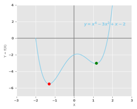
Notice the plot in the Figure.5 above has two minimum points - the one with the red dot and the other with the green dot. The one with the red dot is referred to as the GLOBAL MINIMUM, while the one with the green dot is known as the LOCAL MINIMUM.
The gradient descent algorithm can get into an interesting situation and predict very different function minimum based on where the initial random value for $min$ falls - green dot if the $min$ value is in the interval $(0.2, 2.0)$ and red dot if the $min$ value is in the interval $(0.0, -2.0)$.
Now for a more interesting case, consider the polynomial function $2.sin(x) - 3.cos(\sqrt{5}.x)$. The following illustration shows plot for this trigonometric function:
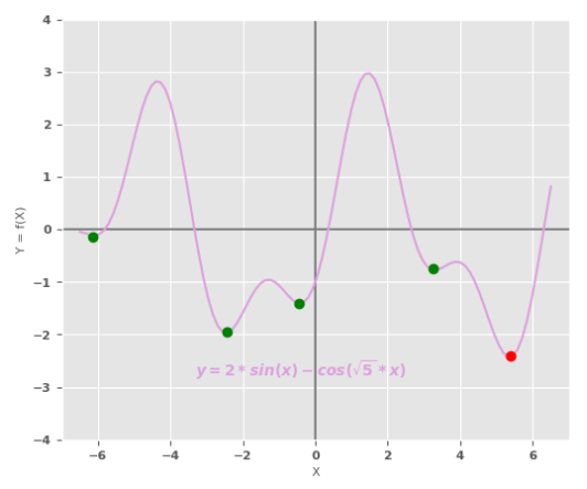
As is evident from the plot in the Figure.6 above, there are more than two minimums. The lowest minimum is referred to as the GLOBAL MINIMUM identified by the red dot, while the remaining ones are known as the LOCAL MINIMUM marked by the green dots.
When there are many LOCAL MINIMUMs, sometimes the gradient descent algorithm may identify a sub-optimal LOCAL MINIMUM.
Until this point, we looked at functions with one variable $x$ in a 2-dimensional space. Let us now look at functions in a 3-dimensional space with two variables.
The following illustration shows the 3-dimensional plot for the function $y = x_1^2 + x_2^2 - 2$ with two variable $x_1$ and $x_2$, with a view from a top angle:
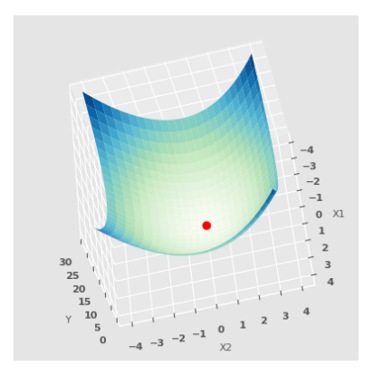
The red dot is the MINIMUM point, which is easy to visualize from the 3-dimensional plot above in Figure.7.
Now, the question one would have is - how does one find the LOCAL MINIMUM for a function with more than one variable (Multivariate Function) as in the above case ???
Once again, Calculus to the rescue with a small twist - we make use of Partial Derivatives !!!
With partial derivatives, one would find the derivative of the multivariate function with respect to each of the variables, treating the remaining variables as constants. Therefore, the gradient of the multivariate function, denoted as $\nabla$, is nothing more than a vector of all the partial derivatives.
As as example, for our multivariate function (from the above) with two variables $x_1$ and $x_2$, its gradient is the vector $\nabla = [\Large{\frac{\partial{f}}{\partial{x_1}}}$$\:\Large{\frac{\partial{f}}{\partial{x_2}}}$ $] = [2.x_1\:2.x_2]$.
The MINIMUM of the multivariate function occurs when the derivative of that function is equal to a ZERO VECTOR (a vector with ZEROs).
For our multivariate function, the minimum is computed as follows:
$[2.x_1\:2.x_2] = [0\:0]$
That is:
$[x_1\:x_2] = [0\:0]$
With that, the following are the high-level steps of the gradient descent algorithm for a higher dimensional space:
Initialize the Maximum Number of Iterations (also called Epochs) and the Learning Rate (denoted using the symbol $\eta$)
Initialize a vector (of size equal to the number of variables in the multivariate function) with random minimum values ($min$)
For each iteration upto the maximum number of iterations (epochs), perform the following steps:
The final minimum vector ($min$) will be an approximation for the minimum of the multivariate function
Backpropagation
Now that we understand the loss function and an approach to minimize a function using gradient descent, we are ready to dive into the details on how to train a neural network for optimal performance by adjusting its weights and biases.
Let us consider a very simple neural network with just an input layer and an output layer with no hidden layer(s). In addition, let will set the bias to ZERO and use an IDENTITY activation function.
The following illustration depicts the simple neural network with the sample data below:
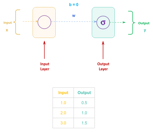
We know the identity activation function $\sigma$ is as given below:
$\sigma = w.x + b$ $..... \color{red}\textbf{(1)}$
where $w$ is the weight and $b$ is the bias.
Since the bias $b$ is equal to $0$, the equation $\color{red}\textbf{(1)}$ becomes:
$\sigma = w.x$ $..... \color{red}\textbf{(2)}$
Also, we know the loss function $L$ is as given below:
$L = (\sigma - y)^2$ $..... \color{red}\textbf{(3)}$
As we know from gradient descent, to minimize the loss function, we need to find its gradient $\nabla L$.
In other words, given that $L$ is dependent on $w$, we need to compute the partial derivative of $L$ with respect to $w$. Note that $L$ is dependent on $\sigma$ (see equation $\color{red}\textbf{(3)}$), which in-turn is dependent on $w$ (see equation $\color{red}\textbf{(2)}$). Therefore, we will need to apply the Chain Rule to find the partial derivative of $L$ with respect to $w$.
That is:
$\nabla L = \Large{\frac{\partial L}{\partial w}}$ $=\Large{\frac{\partial L}{\partial \sigma}}$ $.\Large{\frac{\partial \sigma}{\partial w}}$ $= 2.(\sigma - y).x = 2.(w.x - y).x$ $..... \color{red}\textbf{(4)}$
To minimize the loss from the neural network model, we will need to tweak or adjust the weight $w$ using gradient descent.
In other words:
$w = w - \eta.\nabla L$ $..... \color{red}\textbf{(5)}$
where $\eta$ is the learning rate and let it be set to $0.05$.
Assume the initial random value for $w = 1.2$. Also, let us use $x = 2.0$ as the training data. The following computations demonstrate the iterative training process of our simple neural network model.
Iteration - 1:
With $x = 2.0$ and $w = 1.2$, we find the loss $L = (1.2 * 2.0 - 1.0)^2 = 1.96$ using equation $\color{red}\textbf{(3)}$
To minimize the loss, we find the gradient $\nabla L = 2 * (1.2 * 2.0 - 1.0) * 2.0 = 5.6$ using equation $\color{red}\textbf{(4)}$
Given $\eta = 0.05$, we adjust the weight $w = 1.2 - 0.05 * 5.6 = 0.92$ using equation $\color{red}\textbf{(5)}$
Iteration - 2:
With $x = 2.0$ and $w = 0.92$, we find the loss $L = (0.92 * 2.0 - 1.0)^2 = 0.7$ using equation $\color{red}\textbf{(3)}$
To minimize the loss, we find the gradient $\nabla L = 2 * (0.92 * 2.0 - 1.0) * 2.0 = 3.36$ using equation $\color{red}\textbf{(4)}$
Given $\eta = 0.05$, we adjust the weight $w = 0.92 - 0.05 * 3.36 = 0.75$ using equation $\color{red}\textbf{(5)}$
Iteration - 3:
With $x = 2.0$ and $w = 0.75$, we find the loss $L = (0.75 * 2.0 - 1.0)^2 = 0.25$ using equation $\color{red}\textbf{(3)}$
To minimize the loss, we find the gradient $\nabla L = 2 * (0.75 * 2.0 - 1.0) * 2.0 = 2.02$ using equation $\color{red}\textbf{(4)}$
Given $\eta = 0.05$, we adjust the weight $w = 0.75 - 0.05 * 2.02 = 0.65$ using equation $\color{red}\textbf{(5)}$
Continuing this iterative process, the following illustration shows the values at each iteration:
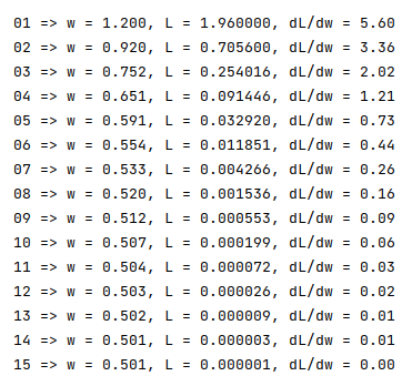
As is evident, the gradient $\nabla L$ is approaching $0.0$ and the value for $w$ is converging to $0.5$, which is the correct value for the weight $w$ of our simple neural network model.
Now that we have a better understanding of how a very simple neural network works, let us build on it for a better intuition on how to compute the gradients for the various weights of the neural network.
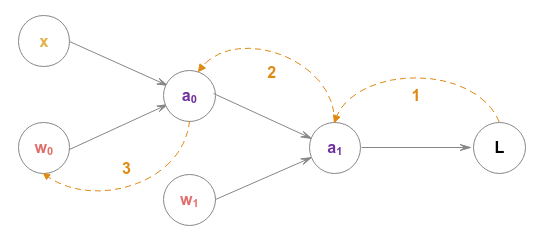
The following illustration depicts another simple neural network with a hidden layer:
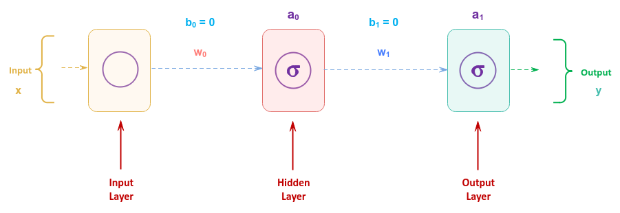
The two weights of the neural network are $w_0$ and $w_1$ respectively. Also, we will set the two biases ($b_0$ and $b_1$) to ZERO. Note that we represent the two activation functions as $a_0$ and $a_1$ for simplicity.
The following illustration depicts the above neural network as a computational graph:
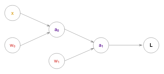
The above computational graph makes it easy to understand the various gradients.
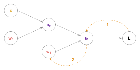
For example, to find the gradient of the loss function $L$ with respect to the weight $w_1$, we use the chain rule as follows:
$\Large{\frac{\partial L}{\partial w_1}}$ $= \Large{\frac{\partial L}{\partial a_1}}$ $.\Large{\frac {\partial a_1}{\partial w_1}}$
The above chain rule is depicted in the following illustration:
Similarly, to find the gradient of the loss function $L$ with respect to the weight $w_0$, we use the chain rule as follows:
$\Large{\frac{\partial L}{\partial w_0}}$ $= \Large{\frac{\partial L}{\partial a_1}}$ $.\Large{\frac {\partial a_1}{\partial a_0}}$ $.\Large{\frac{\partial a_0}{\partial w_0}}$
The above chain rule is depicted in the following illustration:
With all the basics firmed up, it becomes evident that the gradients from a layer be propagated backwards to the previous layer(s) in order to efficiently adjust the weights of the neural network. Hence the approach is known as Backpropagation.
For the final home stretch, let us consider the following illustration of the neural network with an input layer with two inputs, two hidden layers each consisting of two neurons, and an output layer with two outputs:
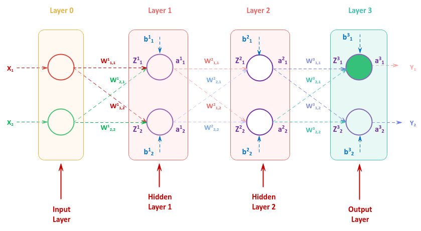
The illustration above in Figure.13 may appear ver complex with lots of letters with exponent and subscript numbers. Let us first break that down as follows:
The number in the exponent such as $w^l$ represents the layer number $l$
The two number subscript such as $w_{j, k}$ represent the input $j$ and the neuron $k$
The letter $w^l_{j, k}$ represents the weight associated with the input $j$ to neuron $k$ in the layer $l$
The letter $b^l_k$ represents the bias to neuron $k$ in the layer $l$
The letter $z^l_k$ represents the input computation $\sum w^l_{j, k}.x^l_j + b^l_k$ going into neuron $k$
The letter $a^l_k$ represents the output from the activation function of neuron $k$
Let us consider the output from the first neuron in the output layer as highlighted in Figure.13 above (in green).
To find the influence of the weight $w^3_{1,1}$ on the loss $L$, we have to look at the following computational graph:
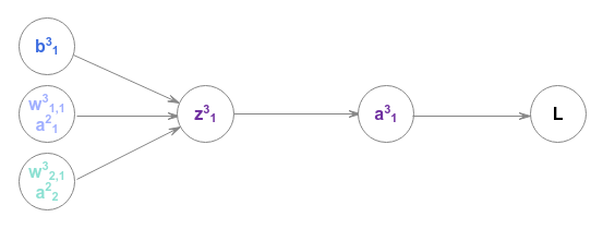
The gradient of the loss $L$ with respect to the weight $w^3_{1,1}$ can be computed using the chain rule as follows:
$\Large{\frac{\partial L}{\partial w^3_{1,1}}}$ $= \Large{\frac{\partial L}{\partial a^3_1}}$ $.\Large{\frac{\partial a^3_1}{\partial z^3_1}}$ $.\Large{\frac{\partial z^3_1}{\partial w^3_{1,1}}}$ $..... \color{red} \textbf{(6)}$
To find the influence of the weight $w^2_{2,1}$ on the loss $L$, we have to look at the following computational graph:
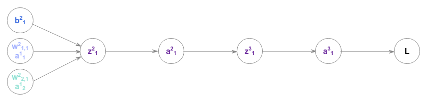
The gradient of the loss $L$ with respect to the weight $w^2_{2,1}$ can be computed using the chain rule as follows:
$\Large{\frac{\partial L}{\partial w^2_{2,1}}}$ $= \Large{\frac{\partial L}{\partial a^3_1}}$ $.\Large{\frac{\partial a^3_1}{\partial z^3_1}}$ $.\Large{\frac{\partial z^3_1}{\partial a^2_1}}$ $.\Large{\frac{\partial a^2_1}{\partial z^2_1}}$ $.\Large{\frac{\partial z^2_1}{\partial w^2_{2,1}}}$ $..... \color{red}\textbf{(7)}$
Some of the gradients in equation $\color{red}\textbf{(7)}$ are already computed in the equation $\color{red}\textbf{(6)}$ and can be propagated backwards for more efficient computation. This pattern repeats itself for the other weights and biases as well.
References