
Figure.1
| PolarSPARC |
Feature Extraction for Natural Language Processing
| Bhaskar S | 02/05/2023 |
Overview
In the article, Basics of Natural Language Processing using NLTK, we introduced the basic concepts in Natural Language Processing (or NLP for short).
The realm of NLP deals with the processing and analysis of the unstructured textual data. In order to extract any kind of meaningful information and/or insights from the unstructured text data, one will have to employ some kind of Machine Learning approach. But, all the Machine Learning approaches ONLY deal with features that have numerical values.
For example, in order to perform any kind of document classification on a corpus (a collection of text documents), one will have to convert each of the text document in the corpus to a set of numerical features (numerical vector) and them perform the classification.
The process of converting a text document to a vector of numbers is often referred to as Feature Extraction or Word Embedding.
The following are some of the basic encoding approaches used in NLP, to convert a text document into a numerical vector:
One-Hot Encoding
Bag of Words
Term Frequency - Inverse Document Frequency
Installation and Setup
Please refer to the article Basics of Natural Language Processing using NLTK for the environment installation and setup.
Open a Terminal window in which we will excute the various commands.
To launch the Jupyter Notebook, execute the following command in the Terminal:
$ jupyter notebook
To set the correct path to the nltk data packages, run the following statement in the Jupyter cell:
nltk.data.path.append("/home/alice/nltk_data")
To initialize a tiny corpus containing 3 sentences for ease of understanding, run the following statements in the Jupyter cell:
['She likes to swim.', 'He loves to read.', 'They like to bike.']
sentences
The following would be a typical output:
To initialize an instance of a word tokenizer, run the following statements in the Jupyter cell:
from nltk.tokenize import WordPunctTokenizer
tokenizer = WordPunctTokenizer()
To normalize the documents in our tiny corpus, run the following statements in the Jupyter cell:
for i in range(len(sentences)):
tokens = tokenizer.tokenize(sentences[i])
words = [word.lower() for word in tokens if word.isalpha()]
sentences[i] = ' '.join(words)
sentences
The following would be a typical output:

One of the IMPORTANT steps in the feature extraction process is to extract all the unique words from the corpus. This typically implies only root words and getting rid of all the rest including punctuations, stop words, etc.
Given our tiny corpus, we will NOT exclude the stop words.
To extract all the unique words from our tiny corpus, run the following statements in the Jupyter cell:
all_words = []
for sentence in sentences:
tokens = tokenizer.tokenize(sentence)
all_words.extend(tokens)
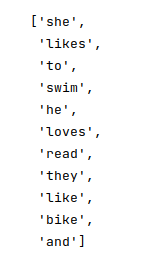
words = sorted(set(all_words), key=all_words.index)
words
The following would be a typical output:
One-Hot Encoding
In the One-Hot Encoding model, a text document in the corpus is encoded as a vector of 1's for each of the unique words from the corpus that is present in the current document. The words not present in the current document are encoded as 0's.
For example, the third sentence from our tiny corpus is encoded as the following vector:
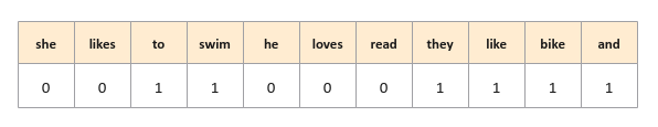
Notice from Figure.4 above, the One-Hot Encoding model DOES NOT maintain the order of the words from the document (the third sentence from out tiny corpus).
For a given corpus, the One-Hot Encoding model outputs a sparse matrix, where the rows represent the documents in the corpus, while the columns are the unique words from the corpus.
To create the One-Hot Encoding sparse matrix for our tiny corpus, run the following statements in the Jupyter cell:
from sklearn.feature_extraction.text import CountVectorizer
model = CountVectorizer(binary=True, vocabulary=words)
matrix = model.fit_transform(sentences).toarray()
one_hot_words = pd.DataFrame(data=matrix, columns=words)
one_hot_words
The following would be a typical output:
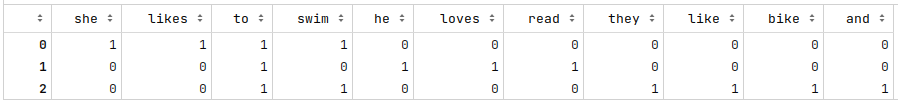
The following are some of the drawbacks of the One-Hot Encoding model:
For a very large corpus, the model performs poorly due to space and time complexity
The model does not preserve the order of the words in the document, thereby losing semantic details
The model only captures if a word is present or not in a document, but not the word frequency, losing some useful information
Bag of Words
The Bag of Words (BoW for short) model improves on the One-Hot Encoding model by capturing the frequency of each of the unique words from the corpus in the current document.
For example, the third sentence from our tiny corpus is encoded as the following vector:
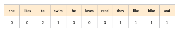
Notice from Figure.6 above, the BoW model encodes a count of 2 for the word to for the third sentence from out tiny corpus.
To create the BoW sparse matrix for our tiny corpus, run the following statements in the Jupyter cell:
from sklearn.feature_extraction.text import CountVectorizer
model = CountVectorizer(vocabulary=words)
matrix = model.fit_transform(sentences).toarray()
bag_of_words = pd.DataFrame(data=matrix, columns=words)
bag_of_words
The following would be a typical output:
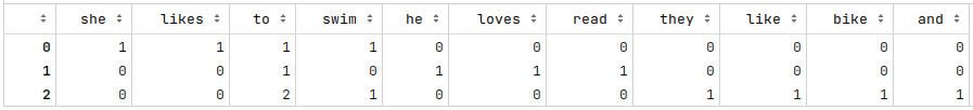
The following are some of the drawbacks of the BoW model:
Frequently occuring words in a document tend to obscure the real intent of the document
For a very large corpus, the model performs poorly due to space and time complexity
The model does not preserve the order of the words in the document, hence losing contextual details
Term Frequency - Inverse Document Frequency
The Term Frequency - Inverse Document Frequency (or TF-IDF for short) model builds on the BoW model. Instead of using a raw word frequency, it uses a statistical measure to determine the relevance of each of the unique words from the corpus with respect to a document in the corpus.
Notice that this model is made up of two very important measures - the Term Frequency and the Inverse Document Frequency.
The Term Frequency, denoted as $TF(w)$, measures the frequency of the word $f(w)$ with respect to the total number of words $F(d)$ in the current document $d$.
In mathematical terms:
$TF(w) = \Large{\frac{f(w)}{F(d)}}$
The Inverse Document Frequency, denoted as $IDF(w)$, measures how common or rare the word $w$ is across the documents in the corpus.
In other words, it is the ratio of the total number of documents in the corpus $N(d)$ to the total number of documents with the word $w$ in the corpus $N(w)$.
In mathematical terms:
$IDF(w) = \Large{\frac{N(d)}{N(w)}}$
If the number of documents in the corpus $N(d)$ is very large, then $IDF(w)$ will be large. To manage this, one typically uses a Logarithmic scale.
In other words:
$IDF(w) = log_e($ $\Large{\frac{N(d)}{N(w)}}$ $)$
If a word $w$ appears in all the documents of the corpus, then $IDF(w) = log_e(1) = 0$
If we desire to assign a very low score versus a $0$ when a word $w$ is common across all the documents in the corpus, the equation for $IDF(w)$ can be modified as follows:
$IDF(w) = log_e($ $1 + \Large{\frac{N(d)}{N(w)}}$ $)$
Given we have the measures for the Term Frequency $TF(w)$ and the Inverse Document Frequency $IDF(w)$, the definition for TD-IDF score in mathematical terms is as follows:
$\textit{TD-IDF(w)} = TF(w) * IDF(w)$
For a given corpus, the TF-IDF model outputs a sparse matrix, where the rows represent the documents in the corpus, while the columns are the unique words from the corpus.
To create the TF-IDF sparse matrix for our tiny corpus, run the following statements in the Jupyter cell:
from sklearn.feature_extraction.text import TfidfVectorizer
model = TfidfVectorizer(vocabulary=words)
matrix = model.fit_transform(sentences).toarray()
tf_idf_words = pd.DataFrame(data=matrix, columns=words)
tf_idf_words
The following would be a typical output:

As is evident from Figure.8 above, the word to appears in all the 3 sentences of our tiny corpus and hence gets a lower score.
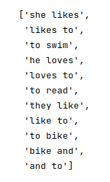
There will be use-cases in which multiple words together (bigrams or trigrams) may provide a better context for the text in the corpus.
To extract all the bigrams from our tiny corpus, run the following statements in the Jupyter cell:
all_bigrams = []
for sentence in sentences:
all_tokens = tokenizer.tokenize(sentence)
bi_tokens = list(nltk.bigrams(all_tokens))
bi_words = [' '.join([w1, w2]) for w1, w2 in bi_tokens]
all_bigrams.extend(bi_words)
all_bigrams = sorted(set(all_bigrams), key=all_bigrams.index)
all_bigrams
The following would be a typical output:
To create the TF-IDF sparse matrix on bigrams for our tiny corpus, run the following statements in the Jupyter cell:
from sklearn.feature_extraction.text import TfidfVectorizer
model = TfidfVectorizer(ngram_range=(2,2), vocabulary=all_bigrams)
matrix = model.fit_transform(sentences).toarray()
tf_idf_bigrams = pd.DataFrame(data=matrix, columns=all_bigrams)
tf_idf_bigrams
The following would be a typical output:

As is evident from Figure.10 above, the bigram to swin appears in all the 2 sentences of our tiny corpus and hence gets a lower score for the third document.
References