Machine Learning - K-Means Clustering using Scikit-Learn

Bhaskar S

07/24/2022

Overview

Clustering is an unsupervised machine learning technique that attempts to group the samples from the unlabeled data set into meaningful clusters.

In other words, the clustering algorithm divides the unlabeled data population into groups, such that the samples within a group are similar to each other.

K-Means Clustering Algorithm

In the following sections, we will unravel the steps behind the K-Means Clustering algorithm using a very simple data set related to Math and Logic scores.

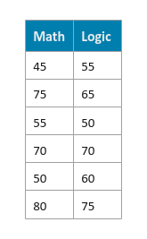
The following illustration displays rows from the simple data set:

Figure.1

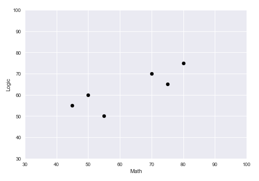
The following illustration shows the plot of the samples from the data set:

Figure.2

Before we get started, the following are some of terminology referenced in this article:

K :: the number of clusters
Centroid :: the average of the samples in a set.

For example, if we have the following three vectors $[4, 5]$, $[6, 7]$, and $[5, 6]$ in a two-dimensional space, then the centroid would be computed as the average of the corresponding elements $\Large{[\frac{4+6+5}{3},\frac{5+7+6}{3}]}$ $= [5, 6]$.

Similarly, if we have the following three vectors $[4, 5, 6]$, $[6, 7, 8]$, and $[5, 6, 7]$ in a three-dimensional space, then the centroid would be computed as $\Large{[\frac{4+6+5}{3},\frac{5+7+6}{3},\frac{6+8+7}{3}]}$ $= [5, 6, 7]$, and so on
Distance :: the distance between two vectors.

For example, for the two vectors $[4, 5]$ and $[6, 7]$ in a two-dimensional space, the L1 distance (or Manhattan distance) is computed as $\lvert 4 - 6 \rvert + \lvert 5 - 7 \rvert = 4$.

The L2 distance (or Euclidean distance) is computed as $\sqrt{(4 - 6)^2 + (5 - 7)^2} = \sqrt{8} = 2.83$
Inertia :: the sum of squared errors between each of the samples in a cluster.

For example, in a two-dimensional space, if the two vectors $[4, 5]$ and $[6, 7]$ are in a cluster with centrod $[5, 6]$, then the value for Inertia is computed as $[(4 - 5)^2 + (5 - 6)^2] + [(6 - 5)^2 + (7 - 6)^2] = [1 + 1] + [1 + 1] = 4$.

As the number of clusters $K$ increases, the corresponding value of Inertia will decrease
Distortion :: the mean value of the Inertia.

For example, in a two-dimensional space, if the two vectors $[4, 5]$ and $[6, 7]$ are in a cluster with centrod $[5, 6]$, then the value for Inertia is computed as $[(4 - 5)^2 + (5 - 6)^2] + [(6 - 5)^2 + (7 - 6)^2] = [1 + 1] + [1 + 1] = 4$. Given there are $2$ samples, the Distortion is $\Large{\frac{4}{2}}$ $= 2$

The following are the steps in the K-Means Clustering algorithm:

Choose the number of clusters $K$. For our simple data set we select $K = 2$
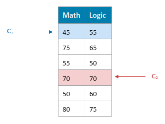
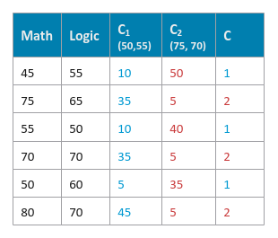
Randomly choose $K$ cluster centroids $C_k$ (where $k = 1 ... K$) from the data set. For our data set, let $C_1 = [45, 55]$ and $C_2 = [70, 70]$.

The following illustration shows the initial centroids for our simple data set:

Figure.3
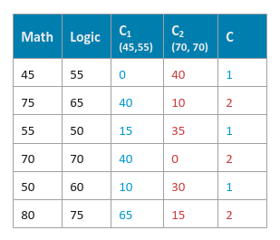
For each sample $X_i$ in the data set, assign the cluster it belongs to. To do that, compute the distance to each of the centroids $C_k$ (where $k = 1 ... K$) and the find the minimum of the distances. If the distance to centroid $C_c$ (where $c \le K$) is the minimum, then assign the sample $X_i$ to the cluster $c$.

The following illustration shows the computed L1 distances and the cluster assignment for our data set:

Figure.4
Compute the new cluster centroids $C_k$ (where $k = 1 ... K$) using the assigned samples $X_i$ to each cluster.

For our data set, the samples $[45, 55]$, $[55, 50]$, and $[50, 60]$ are assigned to cluster $1$. The new cluster centroid for cluster $1$ ($C_1$) would be $\Large{[\frac{45+55+50}{3},\frac{55+50+60}{3}]}$ $= [50, 55]$. Similarly, the new cluster centroid for cluster $2$ ($C_2$) would be $[75, 70]$.
Once again, assign a cluster for each of the samples $X_i$ from the data set.

The following illustration shows the computed L1 distances and the cluster assignment for our data set:

Figure.5
Continue this process of computing the new cluster centroids and assigning samples from the data set to the appropriate clusters until the previous cluster centroids and current cluster centroids are the same.

The following illustration shows the plot of the samples from the data set after the final cluster assignment:

Figure.6

For data sets that are unlabeled, how does one determine the number of clusters $K$ ???

This is where the visual Elbow Method comes in handy. The Elbow Method is a plot of the cluster size $K$ vs the Distortion. From the plot, the idea is to determine the value of $K$, after which the Distortion starts to decrease in smaller steps.

Hands-on Demo

In the following sections, we will demonstrate the use of the K-Means model for clustering (using scikit-learn) by leveraging the Palmer Penguins data set.

The Palmer Penguins includes samples with the following features for the penguin species near the Palmer Station, Antarctica:

species - denotes the penguin species (Adelie, Chinstrap, and Gentoo)
island - denotes the island in Palmer Archipelago, Antarctica (Biscoe, Dream, or Torgersen)
bill_length_mm - denotes the penguins beak length (millimeters)
bill_depth_mm - denotes the penguins beak depth (millimeters)
flipper_length_mm - denotes the penguins flipper length (millimeters)
body_mass_g - denotes the penguins body mass (grams)
sex - denotes the penguins sex (female, male)
year - denotes the study year (2007, 2008, or 2009)

The first step is to import all the necessary Python modules such as, pandas and scikit-learn as shown below:

import pandas as pd
import matplotlib.pyplot as plt
import seaborn as sns
from sklearn.cluster import KMeans

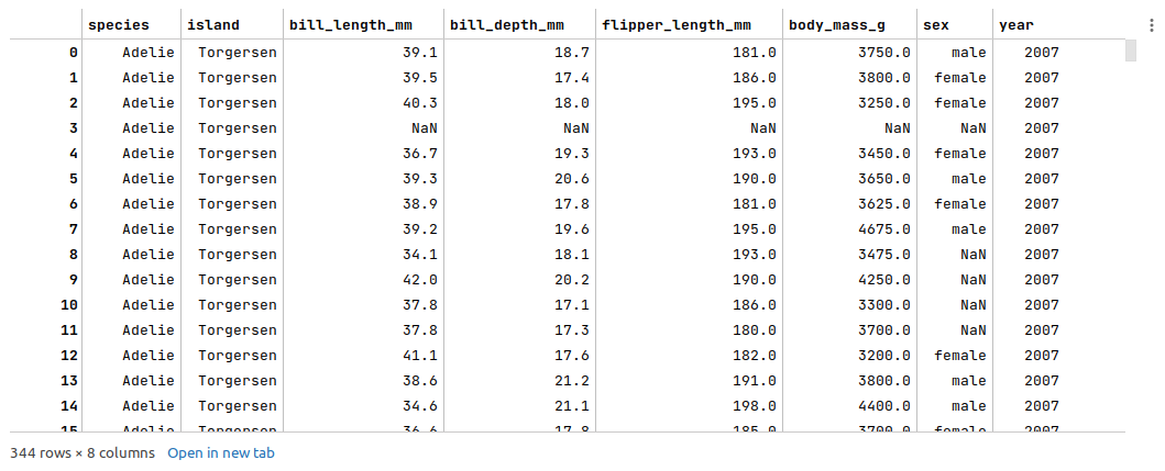
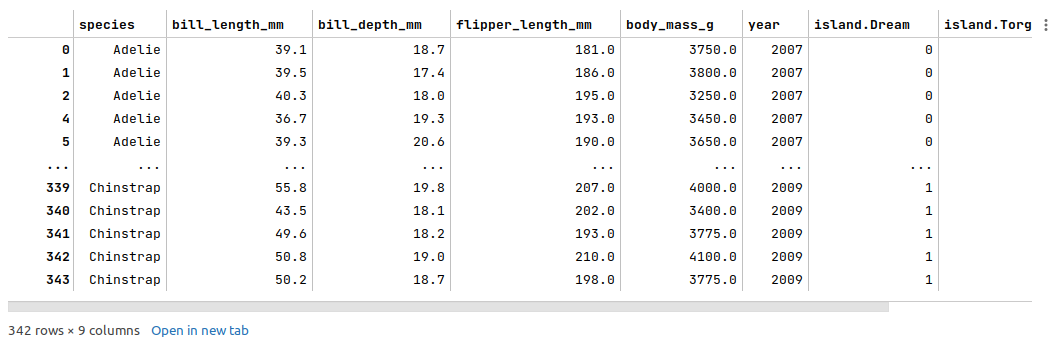
The next step is to load the palmer penguins data set into a pandas dataframe, drop the index column, and then display the dataframe as shown below:

url = 'https://vincentarelbundock.github.io/Rdatasets/csv/palmerpenguins/penguins.csv'
penguins_df = pd.read_csv(url)
penguins_df = penguins_df.drop(penguins_df.columns[0], axis=1)
penguins_df

The following illustration displays few rows from the palmer penguins dataframe:

Figure.7

The next step is to remediate the missing values from the palmer penguins dataframe. Note that we went through the steps to fix the missing values in the article Random Forest using Scikit-Learn, so we will not repeat it here.

For each of the missing values, we perform data analysis such as comparing the mean or (mean + std) values for the features and apply the following fixes as shown below:

penguins_df = penguins_df.drop([3, 271], axis=0)
penguins_df.loc[[8, 10, 11], 'sex'] = 'female'
penguins_df.at[9, 'sex'] = 'male'
penguins_df.at[47, 'sex'] = 'female'
penguins_df.loc[[178, 218, 256, 268], 'sex'] = 'female'

The next step is to display information about the palmer penguins dataframe, such as index and column types, memory usage, etc., as shown below:

penguins_df.info()

The following illustration displays information about the palmer penguins dataframe:

Figure.8

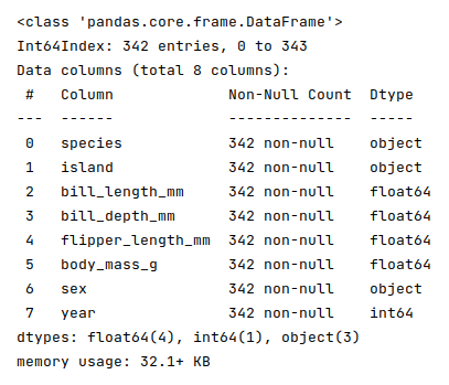
Note that there are no missing values at this point in the palmer penguins dataframe.

The next step is to drop the target variable species from the cleansed palmer penguins dataframe to make it an unlabeled data set as shown below:

penguins_df = penguins_df.drop('species', axis=1)

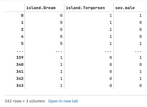
The next step is to create and display dummy binary variables for the two categorical (nominal) feature variables - island and sex from the cleansed palmer penguins dataframe as shown below:

nom_features = ['island', 'sex']
nom_encoded_df = pd.get_dummies(penguins_df[nom_features], prefix_sep='.', drop_first=True, sparse=False)
nom_encoded_df

The following illustration displays the dataframe of all dummy binary variables for the two categorical (nominal) feature variables from the cleansed palmer penguins dataframe:

Figure.9

The next step is to drop the two nominal categorical features and merge the dataframe of dummy binary variables into the cleansed palmer penguins dataframe as shown below:

penguins_df = penguins_df.drop(penguins_df[nom_features], axis=1)
penguins_df = pd.concat([penguins_df, nom_encoded_df], axis=1)
penguins_df

The following illustration displays few columns/rows from the merged palmer penguins dataframe:

Figure.10

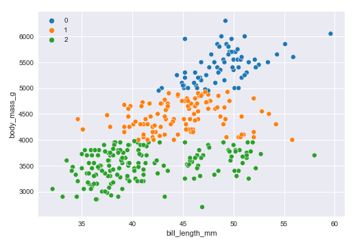
The next step is to initialize the K-Means model class from scikit-learn and train the model using the data set as shown below:

model = KMeans(n_clusters=3, init='random', max_iter=100, random_state=101)
model.fit(penguins_df)

The following are a brief description of some of the hyperparameters used by the KMeans model:

n_clusters - the number of clusters
init - the method to select the initial cluster centroid
max_iter - the maximum number of iterations

The next step is to display a scatter plot of the samples from the palmer penguins data set segregated into the 3 clusters as shown below:

sns.scatterplot(x=penguins_df['bill_length_mm'], y=penguins_df['body_mass_g'], hue=model.labels_, palette='tab10')
plt.show()

The following illustration displays the scatter plot of the 3 clusters:

Figure.11

Demo Notebook

The following is the link to the Jupyter Notebook that provides an hands-on demo for this article:

K-Means Clustering