Figure.1
| PolarSPARC |
Machine Learning - Random Forest using Scikit-Learn
| Bhaskar S | 07/09/2022 |
Overview
In the article Understanding Ensemble Learning, we covered the concept behind the ensemble method Bagging.
Random Forest is a popular machine learning algorithm that leverages the Decision Tree as the base model for the Bagging method.
In other words, the Random Forest machine learning algorithm builds an ensemble of multiple Decision Trees (hence the word Forest) and aggregates the predictions from the multiple trees to make the final prediction.
Random Forest
The Random Forest algorithm uses both bootstrapping of samples as well as selecting $\sqrt{N}$ random feature variables while creating an ensemble of Decision Trees. Without the random feature variable selection, all the trees in the ensemble will have the same root node and similar tree structure. It is possible that some feature variables are not considered. Hence the reason for the random selection of $\sqrt{N}$ feature variables in each of the decision tree so that in the end we will have included all the feature variables.
In this following sections, we will demonstrate the use of the Random Forest model for classification (using scikit-learn) by leveraging the Palmer Penguins data set.
The Palmer Penguins includes samples with the following features for the penguin species near the Palmer Station, Antarctica:
species - denotes the penguin species (Adelie, Chinstrap, and Gentoo)
island - denotes the island in Palmer Archipelago, Antarctica (Biscoe, Dream, or Torgersen)
bill_length_mm - denotes the penguins beak length (millimeters)
bill_depth_mm - denotes the penguins beak depth (millimeters)
flipper_length_mm - denotes the penguins flipper length (millimeters)
body_mass_g - denotes the penguins body mass (grams)
sex - denotes the penguins sex (female, male)
year - denotes the study year (2007, 2008, or 2009)
The first step is to import all the necessary Python modules such as, pandas, matplotlib, seaborn, and scikit-learn as shown below:
import pandas as pd
import matplotlib.pyplot as plt
import seaborn as sns
from sklearn.model_selection import train_test_split
from sklearn.ensemble import RandomForestClassifier
from sklearn.metrics import accuracy_score
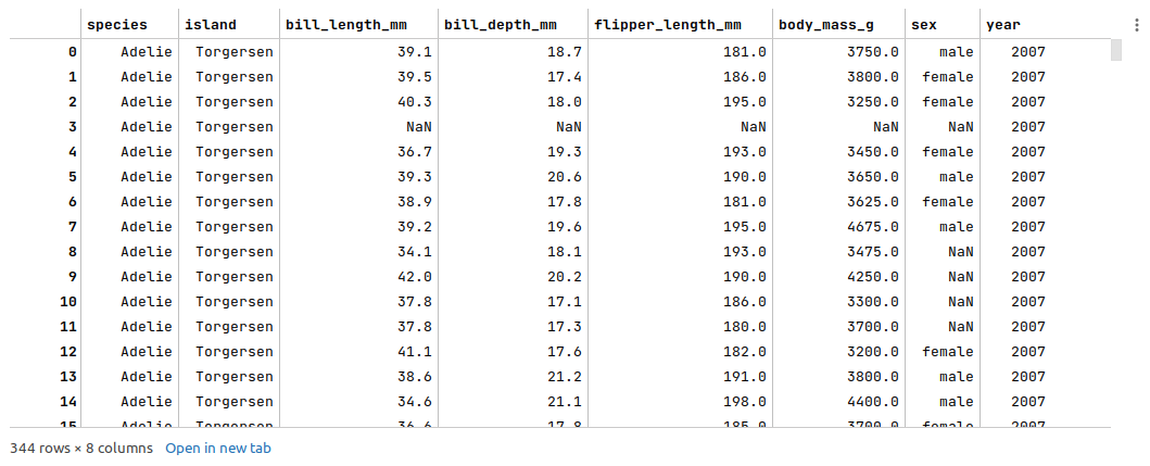
The next step is to load the palmer penguins data set into a pandas dataframe, drop the index column, and then display the dataframe as shown below:
url = 'https://vincentarelbundock.github.io/Rdatasets/csv/palmerpenguins/penguins.csv'
penguins_df = pd.read_csv(url)
penguins_df = penguins_df.drop(penguins_df.columns[0], axis=1)
penguins_df
The following illustration displays few rows from the palmer penguins dataframe:
The next step is to display information about the palmer penguins dataframe, such as index and column types, missing (null) values, memory usage, etc., as shown below:
penguins_df.info()
The following illustration displays information about the palmer penguins dataframe:
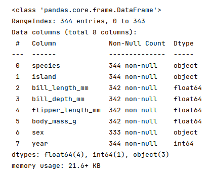
There are a few missing values, so we will identify and remediate them in the following steps.
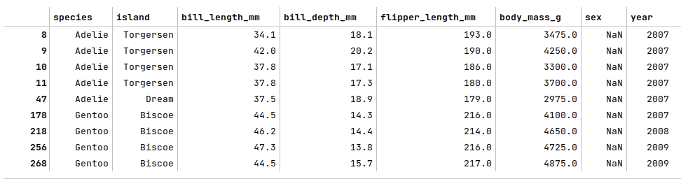
The next step is to display the rows from the palmer penguins dataframe with missing values as shown below:
penguins_df[penguins_df['sex'].isnull()]
The following illustration displays the rows with missing values from the palmer penguins dataframe:
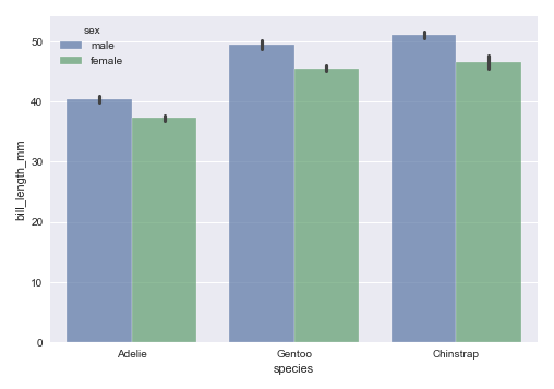
The next step is to display a bar plot between the target feature species and the feature bill_length_mm using the palmer penguins dataframe as shown below:
sns.barplot(data=penguins_df, x='species', y='bill_length_mm', hue='sex', alpha=0.7)
plt.show()
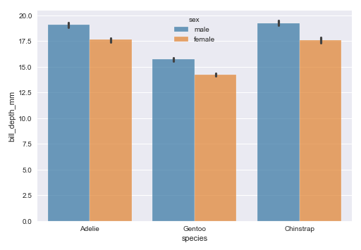
The following illustration shows the bar plot between the target feature species and the feature bill_length_mm using the palmer penguins dataframe:
The next step is to display a bar plot between the target feature species and the feature bill_depth_mm using the palmer penguins dataframe as shown below:
sns.barplot(data=penguins_df, x='species', y='bill_depth_mm', hue='sex', palette='tab10', alpha=0.7)
plt.show()
The following illustration shows the bar plot between the target feature species and the feature bill_depth_mm using the palmer penguins dataframe:
The next step is to display a bar plot between the target feature species and the feature body_mass_g using the palmer penguins dataframe as shown below:
sns.barplot(data=penguins_df, x='species', y='body_mass_g', hue='sex', palette='mako', alpha=0.7)
plt.show()
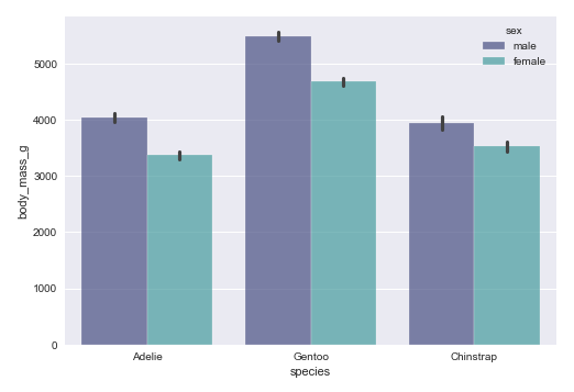
The following illustration shows the bar plot between the target feature species and the feature body_mass_g using the palmer penguins dataframe:
The next step is to display the summary statistics for the rows where the species is 'Adelie' and the island is 'Torgesen' from the palmer penguins dataframe as shown below:
df = pdf[(pdf['species'] == 'Adelie') & (pdf['island'] == 'Torgersen')].groupby('sex').describe()
df.T
The following illustration displays the summary statistics for the selected rows from the palmer penguins dataframe:
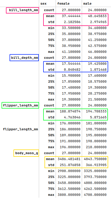
Looking at the plots from Figure.4, Figure.5, Figure.6 and comparing the mean or (mean + std) values from Figure.7 above to the rows where the species is 'Adelie' and the island is 'Torgesen', we can infer that rows at index 8, 10, and 11 are 'female', while the row at index 9 is a 'male'. We apply the fixes as shown below:
penguins_df.loc[[8, 10, 11], 'sex'] = 'female'
penguins_df.at[9, 'sex'] = 'male'
The next step is to display the summary statistics for the rows where the species is 'Adelie' and the island is 'Dream' from the palmer penguins dataframe as shown below:
df = pdf[(pdf['species'] == 'Adelie') & (pdf['island'] == 'Dream')].groupby('sex').describe()
df.T
The following illustration displays the summary statistics for the selected rows from the palmer penguins dataframe:
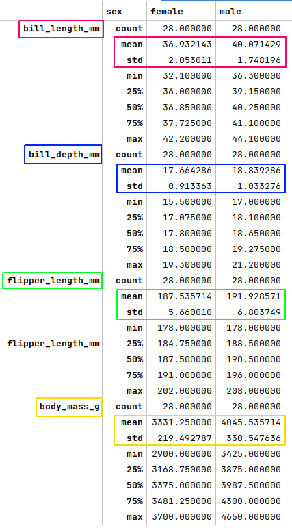
Looking at the plots from Figure.4, Figure.5, Figure.6 and comparing the mean or (mean + std) values from Figure.8 above to the row where the species is 'Adelie' and the island is 'Dream', we can infer that row at index 47 is 'female'. We apply the fix as shown below:
penguins_df.at[47, 'sex'] = 'female'
The next step is to display the summary statistics for the rows where the species is 'Gentoo' and the island is 'Biscoe' from the palmer penguins dataframe as shown below:
df = pdf[(pdf['species'] == 'Gentoo') & (pdf['island'] == 'Biscoe')].groupby('sex').describe()
df.T
The following illustration displays the summary statistics for the selected rows from the palmer penguins dataframe:
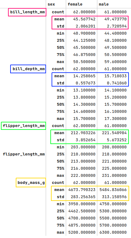
Looking at the plots from Figure.4, Figure.5, Figure.6 and comparing the mean or (mean + std) values from Figure.9 above to the rows where the species is 'Gentoo' and the island is 'Biscoe', we can infer that the rows at index 178, 218, 256, and 268 are 'female'. We apply the fix as shown below:
penguins_df.loc[[178, 218, 256, 268], 'sex'] = 'female'
At this point, all the missing values have been addressed and we are ready to move to the next steps.
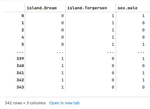
The next step is to create and display dummy binary variables for the two categorical (nominal) feature variables - island and sex from the cleansed palmer penguins dataframe as shown below:
nom_features = ['island', 'sex']
nom_encoded_df = pd.get_dummies(penguins_df[nom_features], prefix_sep='.', drop_first=True, sparse=False)
nom_encoded_df
The following illustration displays the dataframe of all dummy binary variables for the two categorical (nominal) feature variables from the cleansed palmer penguins dataframe:
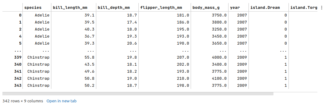
The next step is to drop the two nominal categorical features and merge the dataframe of dummy binary variables into the cleansed palmer penguins dataframe as shown below:
penguins_df2 = penguins_df.drop(penguins_df[nom_features], axis=1)
penguins_df3 = pd.concat([penguins_df2, nom_encoded_df], axis=1)
penguins_df3
The following illustration displays few columns/rows from the merged palmer penguins dataframe:
The next step is to split the palmer penguins dataframe into two parts - a training data set and a test data set. The training data set is used to train the ensemble model and the test data set is used to evaluate the ensemble model. In this use case, we split 75% of the samples into the training dataset and remaining 25% into the test dataset as shown below:
X_train, X_test, y_train, y_test = train_test_split(penguins_df3, penguins_df3['species'], test_size=0.25, random_state=101)
X_train = X_train.drop('species', axis=1)
X_test = X_test.drop('species', axis=1)
The next step is to initialize the Random Forest model class from scikit-learn and train the model using the training data set as shown below:
model = RandomForestClassifier(max_depth=4, n_estimators=64, random_state=101)
model.fit(X_train, y_train)
The following are a brief description of some of the hyperparameters used by the Random Forest model:
max_depth - the maximum depth of each of the decision trees in the ensemble
n_estimators - the total number of trees in the ensemble. The typical suggested value is between 64 and 128. The default value is 100
max_features - the number of features to randomly select for each tree in the ensemble. The default is $\sqrt{N}$, where $N$ is the number of features in the data set
oob_score - flag that indicates if the out-of-bag samples must be used for validation. Given that we are using a train and test split, this is not necessary. The default is false
The next step is to use the trained model to predict the species using the test dataset as shown below:
y_predict = model.predict(X_test)
The next step is to display the accuracy score for the model performance as shown below:
accuracy_score(y_test, y_predict)
The following illustration displays the accuracy score for the model performance:
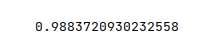
From the above, one can infer that the model seems to predict with accuracy.
Hands-on Demo
The following is the link to the Jupyter Notebook that provides an hands-on demo for this article:
References