Machine Learning - Linear Regression using Scikit-Learn

Machine Learning - Linear Regression using Scikit-Learn - Part 2

Bhaskar S

03/26/2022

Overview

Scikit-Learn is a popular open-source Python library that provides support for the various machine learning algorithms via a simple and consistent API interface.

In this article, we will demonstrate an example for both the Simple Linear Regression and the Multiple Linear Regression using scikit-learn.

We will leverage the popular Auto MPG dataset for the demonstration.

Simple Linear Regression

For simple linear regression, we will demonstrate 3 models in the hands-on demo:

displacement VS mpg
horsepower VS mpg
weight VS mpg

The first step is to import all the necessary Python modules such as, matplotlib, pandas, and scikit-learn as shown below:

import pandas as pd
import matplotlib.pyplot as plt
from sklearn.model_selection import train_test_split
from sklearn.linear_model import LinearRegression
from sklearn.metrics import r2_score

The next step is to load the auto mpg dataset into a pandas dataframe and assign the column names as shown below:

url = 'https://archive.ics.uci.edu/ml/machine-learning-databases/auto-mpg/auto-mpg.data'
auto_df = pd.read_csv(url, delim_whitespace=True)
auto_df.columns = ['mpg', 'cylinders', 'displacement', 'horsepower', 'weight', 'acceleration', 'model_year', 'origin', 'car_name']

The next set of steps involves making sense of the data and fixing data quality issues, such as fixing data type issues, eliminating (or replacing) missing values, extracting important features variables, etc. These steps are in the realm of Exploratory Data Analysis.

The next step is to explore the data types of the columns in the auto mpg dataframe as shown below:

auto_df.dtypes

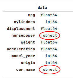
The following illustration shows the data types of the columns of the the auto mpg dataset:

Figure.1

The data types for the columns horsepower and car_name are highlighted to indicate they need to be fixed appropriately.

The next step is to fix the data types of the identified columns in the auto mpg dataframe as shown below:

auto_df.horsepower = pd.to_numeric(auto_df.horsepower, errors='coerce')
auto_df.car_name = auto_df.car_name.astype('string')
auto_df.dtypes

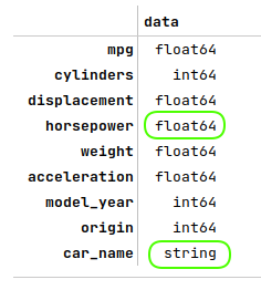
The following illustration shows the corrected data types for the columns of the auto mpg dataset:

Figure.2

The next step is to display information about the auto mpg dataframe, such as index and column types, missing (null) values, memory usage, etc., as shown below:

auto_df.info()

The following illustration displays information about the auto mpg dataframe:

Figure.3

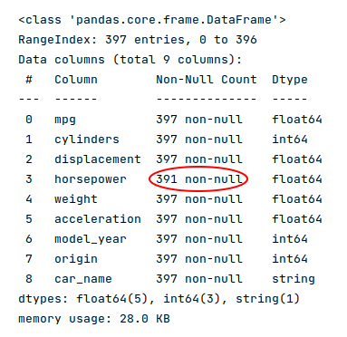
The highlighted part for the horsepower row indicates we are missing some values.

The next step is to display the rows from the auto mpg dataframe with missing values as shown below:

auto_df[auto_df.horsepower.isnull()]

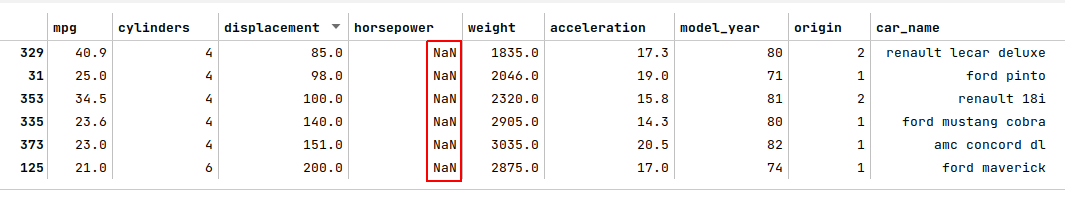
The following illustration displays the rows with missing values from the auto mpg dataframe:

Figure.4

The next step is to eliminate the rows from the auto mpg dataframe with missing values as shown below:

auto_df = auto_df[auto_df.horsepower.notnull()]

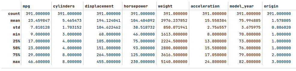
The next step is to display the summary statistics on the various columns of the auto mpg dataframe as shown below:

auto_df.describe()

The following illustration displays the summary statistics on the various columns of the auto mpg dataframe:

Figure.5

At this point, we have completed the basic steps involved in the exploratory data analysis.

The next step is to split the auto mpg dataset into two parts - a training dataset and a test dataset. We use the training dataset to train the regression model and use the test dataset to evaluate the regression model. Typically, the training dataset is about 75% to 80% from the population. We split 75% of the population into the training dataset and 25% into the test dataset as shown below:

X_train, X_test, y_train, y_test = train_test_split(auto_df[['displacement']], auto_df['mpg'], test_size=0.25, random_state=101)

Note that the training and test datasets will contain a RANDOM sample from the population.

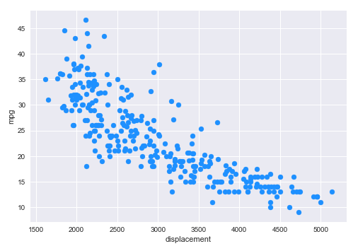
The next step is to display a scatter plot that shows the visual relationship between the data from the columns displacement and mpg from the auto mpg training dataset as shown below:

plt.scatter(X_train, y_train, color='dodgerblue')
plt.xlabel('displacement')
plt.ylabel('mpg')
plt.show()

The following illustration shows the scatter plot between displacement and mpg from the auto mpg training dataset:

Figure.6

The next step is to initialize the desired model class from scikit-learn. When initializing a model, one can specify the various hyperparameters, such as the need to include a y-intercept for the line of best fit, etc. For our demonstration, we will initialize a linear regression model with the line-intercept as shown below:

model1 = LinearRegression(fit_intercept=True)

The next step is to train the model using the training dataset as shown below:

model1.fit(X_train, y_train)

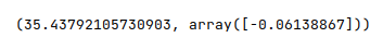
The next step is to display the values for the intercept and the coefficient (the slope) as shown below:

model1.intercept_, model1.coef_

The following illustration displays the values for the intercept and the coefficient (the slope) from the model:

Figure.7

The next step is to use the trained model to predict the mpg using the test dataset as shown below:

y_predict = model1.predict(X_test)

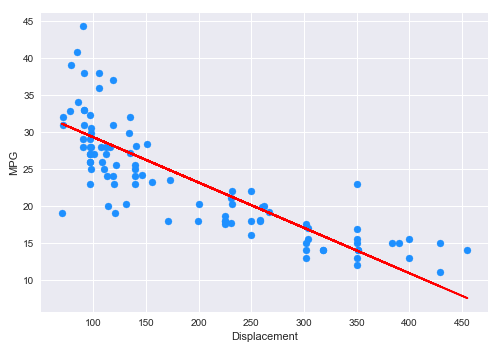
The next step is to display a scatter plot (along with the line of best fit) that shows the visual relationship between the data from the columns displacement and mpg from the auto mpg test dataset as shown below:

plt.scatter(X_test, y_test, color='dodgerblue')
plt.plot(X_test['displacement'], y_predict, color='red')
plt.xlabel('Displacement')
plt.ylabel('MPG')
plt.show()

The following illustration shows the scatter plot (along with the line of best fit) between displacement and mpg from the auto mpg test dataset:

Displacement vs MPG with Regression Line

Figure.8

The final step is to display the $R^2$ value for the model as shown below:

r2_score(y_test, y_predict)

The following illustration displays the $R^2$ value for the model:

Figure.9

We will not go over the other two models here as the process is similar to the above steps and is included in the hands-on demo notebooks.

Multiple Linear Regression

Many of the steps we went over in the simple linear regression section, such as loading the data and performing the basic exploratory data analysis, etc., will be skipped in this section as they are very similar.

The next step is to create the training dataset and a test dataset with the desired feature (or predictor) variables. We create a 75% training dataset and a 25% test dataset with the four feature variables acceleration, displacement, horsepower, and weight as shown below:

X_train, X_test, y_train, y_test = train_test_split(auto_df[['acceleration', 'displacement', 'horsepower', 'weight']], auto_df['mpg'], test_size=0.25, random_state=101)

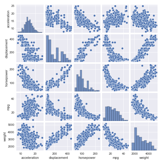
The next step is to display a pair plot that shows the visual relationship between the target and predictor variables from the auto mpg training dataset as shown below:

sns.pairplot(auto_df[['acceleration', 'displacement', 'horsepower', 'mpg', 'weight']], height=1.5)
plt.show()

The following illustration shows the pair plot between the target and predictor variables from the auto mpg training dataset:

Figure.10

The next step is to initialize the linear regression model with the line-intercept as shown below:

model = LinearRegression(fit_intercept=True)

The next step is to train the model using the training dataset as shown below:

model.fit(X_train, y_train)

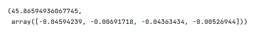
The next step is to display the values for the intercept and the regression coefficients as shown below:

model.intercept_, model.coef_

The following illustration displays the values for the intercept and the regression coefficients from the model:

Figure.11

The next step is to use the trained model to predict the mpg using the test dataset as shown below:

y_predict = model.predict(X_test)

The next step is to display the $R^2$ value for the model as shown below:

r2_score(y_test, y_predict)

The following illustration displays the $R^2$ value for the model:

Figure.12

The final step is to display the adjusted $\bar{R}^2$ value for the model as shown below:

adj_r2_score(X_test, y_test, y_predict)

The following illustration displays the adjusted $\bar{R}^2$ value for the model:

Figure.13

Hands-on Demo

The following are the links to the Jupyter Notebooks that provides an hands-on demo for this article:

References

Machine Learning - Linear Regression - Part 1