Introduction to Statistics - Part 2
In Part 1 of the series, we
introduced the basic concepts of Statistics and explored the measures of central tendency and
measures of dispersion.
In this part of the series, we will introduce concepts around the various probability distributions. This will require
some basic understanding of Permutation
& Combinations as well as
Probability.
A Random Variable denotes a quantitative (numerical) value that is associated with the random
outcome of a statistical experiment.
A Discrete random variable has a finite (a countable) number of outcomes (values) in a given
interval.
A Continuous random variable can assume an infinite (not countable) number of possible outcomes.
A Probability Distribution is a statistical function that describes the probability of occurrence
of each of the possible outcomes of the random variable in a statistical experiment.
Discrete Probability Distribution
A Discrete Probability Distribution lists out each possible value of the discrete random
variable along with its probability. The distribution must satisfy the following conditions:
The mean of a discrete probability distribution is computed using the formula:
\(\mu = \Sigma{x_i}.{P(x_i)}\), where i = 1 to n
The variance of a discrete probability distribution is computed using the formula:
\(\sigma^2 = \Sigma({x_i} - \mu)^2.{P(x_i)}\), where i = 1 to n
The standard deviation of a discrete probability distribution is computed using the formula:
\(\sigma = \sqrt{\Sigma({x_i} - \mu)^2.{P(x_i)}}\), where i = 1 to n
There are two popular discrete probability distributions which are as follows:
Binomial Probability Distribution
A Binomial Probability Distribution is a probability experiment that must satisfy the following
conditions:
-
The experiment has a fixed number of repeated trials represented by n
-
Each of the n trials are independent and repeated under identical conditions (the outcome of one trial does not affect
the outcome of other trials)
-
Each trial has only two possible outcomes - a success (p for probability of success) or as a failure (q for probability
of failure = 1 - p)
-
The probability of a success is the same for each trial
-
The random variable x represents the number of successful outcomes from the n trials
The mathematical formula for binomial probability distribution of exactly x success(es) in n trials is as follows:
\(_{n}C_{x}.p^{x}.q^{n-x} =\) \(\Large{\frac{n!}{(n-x)!x!}}\)\(.p^{x}.q^{n-x}\), where q = (1 - p),
and \(_{n}C_{x}\) = \(\Large{\frac{n!}{(n-x)!x!}}\)
| Example-1 |
Knee surgery has a 90% chance of success. The surgery is performed on 3 patients. What is the probability of the
surgery being successful on exactly 2 patients.
|
|
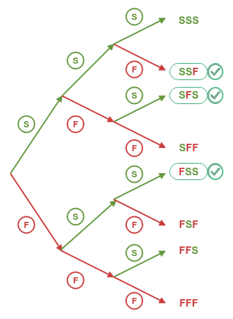
The following tree diagram illustrates the various outcomes (S for success and F for failure) from the 3 surgeries
(experiments):
Outcomes
The probability of success (p) = 90/100 = 9/10.
The probability of failure (q) = 1 - p = 1 - 9/10 = 1/10.
From the illustration above, we observe there are only 3 outcomes that have 2 successful outcomes - SSF, SFS, and
FSS.
The probability for SSF = 9/10 . 9/10 . 1/10 = 81/1000.
The probability for SFS = 9/10 . 1/10 . 9/10 = 81/1000.
The probability for FSS = 1/10 . 9/10 . 9/10 = 81/1000.
Therefore, the probability for exactly 2 successes from the 3 surgeries = 81/1000 + 81/1000 + 81/1000 = 243/1000
= 0.243.
Next, we will compute the probability using the formula: \(\Large{\frac{n!}{(n-x)!x!}}\)\(.p^{x}.q^{n-x}\).
That is, \(\Large{\frac{3!}{(3-2)!2!}}\)\(.(0.9)^{2}.(0.1)^{(3-2)}\) = 3.(0.81) = 0.243.
|
We will look at another example for binomial probability distribution.
| Example-2 |
A survey of U.S. adults found that 70% of them believe that there is a link between playing violent video games and
teens exhibiting violent behavior. An experiment randomly selects 3 adults and asks them about their belief. Find the
probability that at least 2 of them respond YES.
|
|
The number of trials (n) = 3.
The probability of success (p) = 70/100 = 7/10 = 0.7.
The probability of failure (q) = 1 - p = 1 - 7/10 = 3/10 = 0.3.
The number of successful outcomes expected (x) = 2 or 3 (because at least 2 of them responsed YES).
The probability formula is: \(P(x) = \Large{\frac{n!}{(n-x)!x!}}\)\(.p^{x}.q^{n-x}\).
\(P(2) = \Large{\frac{3!}{(3-2)!2!}}\)\(.(0.7)^{2}.(0.3)^{(3-2)}\) = 3.(0.49).(0.3) =
0.441.
\(P(3) = \Large{\frac{3!}{(3-3)!3!}}\)\(.(0.7)^{3}.(0.3)^{(3-3)} = (0.7)^3\) = 0.343.
Therefore, the probability that at least 2 of them respond YES = P(2) + P(3) = 0.441 + 0.343 =
0.784.
|
Poisson Probability Distribution
A Poisson Probability Distribution is a probability experiment that must satisfy the following
conditions:
-
Each trial has only two possible outcomes - the event occurs (success) or the event *DOES NOT* occur (failure)
-
The experiment consists of counting the number of times (x) the event occurs in a given interval of time
-
The probability of the event occuring (success) is the same for each trial
-
The number of occurrences in one interval is independent of the number of occurrences in other intervals
-
The average number of times the event occurs (success) (\(\mu\)) in a given interval is known and is constant
The mathematical formula for poisson probability distribution of exactly x occurrences of the event (success) in an interval
is as follows:
\(P(x,\mu) = e^{-\mu}\).\(\Large{\frac{\mu^x}{x!}}\), where e is the base of the natural logarithm
and is an irrational number that approximately equals 2.71828 and \(\mu\) is the average number of occurrences of the event
per interval.
| Example-3 |
In a city, accidents occur randomly at an average rate of 1.8 per hour. What is the probability of observing more than
2 accidents in a given hour in that city.
|
|
The probability formula is: \(P(x,\mu) = e^{-\mu}\).\(\Large{\frac{\mu^x}{x!}}\).
Given the average number of accidents per hour: \(\mu = 1.8\).
We want to find: \(P(x >= 2, \mu) = P(2, \mu) + P(3, \mu) + ...\).
This can also be written as: \(1 - P(x < 2, \mu) = 1 - P(0, \mu) - P(1, \mu)\).
That is, 1 - \(e^{-1.8}\).\(\Large{\frac{1.8^0}{0!}}\) - \(e^{-1.8}\).\(\Large{\frac{1.8^1}{1!}}\).
That is, 1 - \(e^{-1.8}\) - \(e^{-1.8}.(1.8)\).
We find that \(e^{-1.8} \approx 0.1653\).
Therefore, \(P(x >= 2, \mu) = 1 - 0.1653 - 0.2975 \) = 0.5372.
|
Continuous Probability Distribution
A Continuous Probability Distribution can be described using a graph f(x) that represents a
Probability Density Function. The probability density function describes the likelihood that
the values of the continuous random variable (x) fall within a given interval. The distribution must satisfy the following
conditions:
-
Because a continuous random variable (x) can have infinite values, the probability that the continuous random variable
takes a specific value is 0
-
The probability that the continuous random variable (x) assumes a value within an interval, say P(A ≤ x ≤ B), is
defined as the area under the graph f(x) between the points A and B
-
The entire area under the graph f(x) over all values of the continuous random variable (x) must equal 1
The most popular continuous probability distribution is the Normal Distribution (which is
also referred to as the Gaussian Distribution).
A Normal Distribution is a continuous probability distribution for a continuous random variable
(x) that must satisfy the following conditions:
-
The graph f(x) (referred to as a Normal Curve) is bell-shaped curve (with a long tail)
and is symmetrical around the mean
-
The mean, median, and mode are equal
-
The total area under the normal curve is equal to 1
-
68% of the area under the normal curve falls within 1 standard deviation of the mean
-
95% of the area under the normal curve falls within 2 standard deviations of the mean
-
99.7% of the area under the normal curve falls within 3 standard deviations of the mean
The following diagram illustrates a typical normal curve:
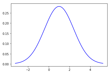
Normal Curve
The mathematical equation for a normal probability density function f(x) with a mean of \(\mu\) and standard deviation of
\(\sigma\) is given as follows:
\(f(x,\mu,\sigma) =\)\(\Large{\frac{1}{\sigma\sqrt{2\pi}}}\).\(e^{-\frac{1}{2}(\frac{x -
\mu}{\sigma})^2}\), where e is the base of the natural logarithm and is an irrational number that approximately equals 2.71828
and \(\pi\) is an irrational number that approximately equals 3.14159.
For each mean and standard deviation, there is a different normal distribution. In other words, there are infinitely many
normal distributions with different means and standard deviations. The normal distribution with a mean of 0 and a standard
deviation of 1 is called the Standard Normal Distribution.
The following diagram illustrates the standard normal curve for the standard normal distribution:
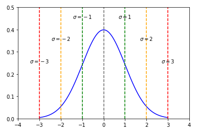
Standard Normal Curve
The horizontal scale (x-axis) of the standard normal curve of the standard normal distribution corresponds to what is called
the Z-scores. A Z-score is a measure that
indicates the number of standard deviations a value (x) lies from the mean.
The Z-score for a given x value can be computed using the following formula:
\(Z = \Large{\frac{x - \mu}{\sigma}}\).
In general, a Z-score of more than 3 standard deviations from the mean is considered an outlier.
For a random variable x that is normally distributed, one can find the probability that x will lie in the given interval
by calculating the area under the normal curve for the given interval. To find the area under any normal curve, we first
have to convert the upper and lower bounds of the given interval to Z-scores. We then use the standard normal distribution
to find the area under the curve.
The following illustration shows the negative Z-scores table that correspond to values which are less than the mean:
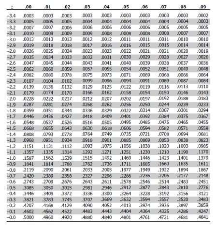
Negative Z-Scores
The following illustration shows the positive Z-scores table that correspond to values which are greater than the mean:
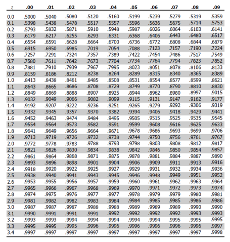
Positive Z-Scores
Let us look at a very simple example to find the area to the left of a given Z-score value.
| Example-4 |
Find the area under the standard normal curve to the left of z = -0.99
|
|
The following normal curve illustrates the shaded area to the left of Z = -0.99:
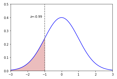
Left of Z = -0.99
From the Negative Z-Scores table above, we can find that area to the left is equal to
0.1611.
|
Now, let us look at another simple example to find the area to the right of a given Z-score value.
| Example-5 |
Find the area under the standard normal curve to the right of z = 1.06
|
|
The following normal curve illustrates the shaded area to the right of Z = 1.06:
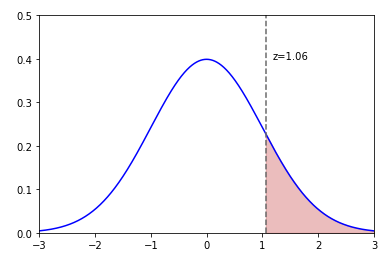
Right of Z = 1.06
From the Positive Z-Scores table above, we can find that area to the left is equal to 0.8554.
To find the area to the right, we need to subtract from the whole area of 1.
That is, 1 - 0.8554 = 0.1446.
|
Now, we look at one other simple example to find the area between the given two Z-score values.
| Example-6 |
Find the area under the standard normal curve between z = -1.5 and z = 1.25
|
|
The following normal curve illustrates the shaded area between z = -1.5 and z = 1.25:
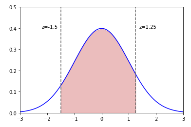
Between z = -1.5 and z = 1.25
(A) From the Negative Z-Scores table above, we can find that area to the left of Z = -1.5 is equal to 0.0668.
(B) From the Positive Z-Scores table above, we can find that area to the left of Z = 1.25 is equal to 0.8944.
To find the area between z = -1.5 and z = 1.25, we need to subtract (A) from (B).
That is, 0.8944 - 0.0668 = 0.8276.
|
Finally, we look at a word problem for finding probabilities with the normal distribution.
| Example-7 |
The average speed of vehicles traveling on a highway is 67 miles per hour with a standard deviation of 3.5 miles per
hour. If a vehicle is selected at random, what is the probability that it is violating the speed limit of 70 miles per
hour
|
|
Given, the average speed \(\mu = 67\) and the standard deviation of \(\sigma = 3.5\).
In order to find the probability if a randomly picked vehicle will violate the speed of greater than or equal to 70
miles per hour, we need to normalize using the Z-score.
We know \(z = \Large{\frac{x - \mu}{\sigma}}\) = \(\Large{\frac{70 - 67}{3.5}}\) = 0.8571 \(\approx 0.86\).
The following normal curve illustrates the shaded to the right of the speed of greater than or equal to 70 miles per
hour:
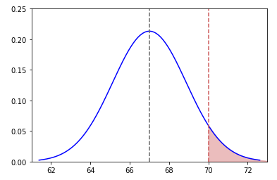
Speed Violation
From the Positive Z-Scores table above, we can find that area to the left of z = 0.86 is equal to 0.8051.
To find the area to the right, we need to subtract from the whole area of 1.
Therefore, the probability that a randomly selected vehicle will violate the speed limit of 70 miles per hour, 1 -
0.8051 = 0.1949.
|