Machine Learning - AdaBoost using Scikit-Learn

In the article Understanding Ensemble Learning, we covered the concept behind the ensemble method Boosting.

AdaBoost (short for Adaptive Boosting) is one of the machine learning algorithms that leverages the Decision Tree as the base model (also referred to as a weak model) for the Boosting method.

In other words, the AdaBoost machine learning algorithm iteratively builds a sequence of Decision Trees, such that each of the subsequent Decision Trees work on the misclassifications from the preceding trees, to arrive at a final prediction.

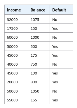
In the following sections, we will unravel the steps behind the AdaBoost algorithm using a very simple hypothetical data set relating to whether someone will default based on their income and current balance.

The following illustration displays rows from the hypothetical defaults data set:

The following are the steps in the AdaBoost algorithm:

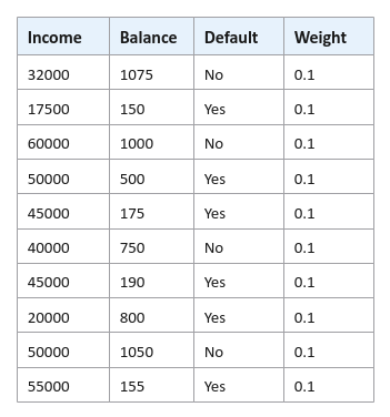
Assign an initial weight (that represents the level of importance) to each of the samples (rows) in the data set. The initial weight $w_0$ for each sample is $\Large{\frac{1}{N}}$, where $N$ is the number of samples. For our hypothetical defaults data set, we have $10$ samples and hence $w_0 = 0.1$ for each sample in the data set as shown below:

Figure.2
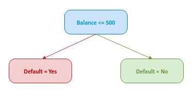
Create a weak base model (a decision stump) from the features (in the data set) with the lowest gini index. Note that a feature selection for the root node depends on the samples in the data set. For our data set, assume the feature Balance is chosen as the root node of the decision stump as shown below:

Figure.3

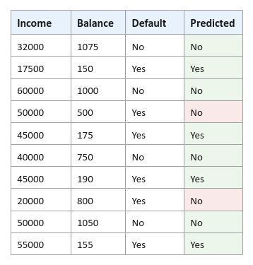
Using the weak model, the following illustration shows the predicted outcome:

Figure.4
Determine the performance coefficient of the weak base model based on the errors the model made.

The Performance Coefficient $\alpha$ of the weak base model is computed as $\gamma * log_e \Large{(\frac{1 - E_t}{E_t})}$, where $\gamma$ is the Learning Rate and $E_t$ is the Total Error.

The Learning Rate controls the level of significance (or contribution) of the weak base model in the ensemble. For this example, we will set the Learning Rate as $\gamma = \Large{\frac{1}{2}}$.

The Total Error $E_t$ is computed as the sum of weights of all the mis-classified data samples by the weak base model. The Total Error value will always be between $0$ and $1$.

For our hypothetical defaults data set, from the Figure.4 above, we see two mis-classifications and hence the Total Error $E_t = 0.1 + 0.1 = 0.2$.

Therefore the Performance Coefficient for our example is $\alpha = \Large{\frac{1}{2}}$ $log_e \Large{(\frac {1 - 0.2}{0.2})}$ $= \Large{\frac{1}{2}}$ $log_e \Large{(\frac{0.8}{0.2})}$ $= 0.5 * log_e(4) = 0.5 * 1.38 = 0.69$.
Adjust the weight of the samples in the data set using the Performance Coefficient, such that the weights for the correctly classified samples are reduced while the weights for the mis-classified samples are increased.

The new weight $w_1$ for correctly classified samples is computed as $w_1 = w_0 * e^{-\alpha}$ and for mis-classified samples is computed as $w_1 = w_0 * e^{\alpha}$.

In general terms, the new weight $w_i$ for correctly classified samples is computed as $w_i = w_{i-1} * e^{-\alpha}$ and for mis-classified samples is computed as $w_i = w_{i-1} * e^{\alpha}$.

For the correctly classified samples $w_1 = 0.1 * e^{-0.69} = 0.1 * 0.5016 = 0.50$.

For the mis-classified samples $w_1 = 0.1 * e^{0.69} = 0.1 * 1.9937 = 0.199$.

The following illustration shows the samples from the data set with adjusted weights:

Figure.5
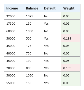
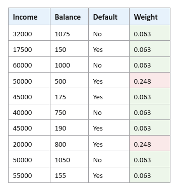
Normalize the weight of the samples in the data set so they all add upto $1$. For this, we divide each of the weights in the data set by the sum of all the weights. The sum of all the weights from the table in Figure.5 from above equals $0.798$. The normalized weight for $0.05$ is $\Large{\frac{0.05}{0.798}}$ $= 0.63$. Similarly, the normalized weight for $0.199$ is $\Large{\frac{0.199}{0.798}}$ $= 0.248$.

The following illustration shows the samples from the data set with normalized weights:

Figure.6
Create a new data set that includes only the samples with the higher weights (can include duplicates). The main idea behind this is that the next weak model will focus on the mis-classified samples.
Go to Step 2 for the next iteration. This process continues until a specified number of weak base models are reached. Note that the iteration will stop early if a perfect prediction state is reached.

In the following sections, we will demonstrate the use of the AdaBoost model for classification (using scikit-learn) by leveraging the Palmer Penguins data set.

The Palmer Penguins includes samples with the following features for the penguin species near the Palmer Station, Antarctica:

species - denotes the penguin species (Adelie, Chinstrap, and Gentoo)
island - denotes the island in Palmer Archipelago, Antarctica (Biscoe, Dream, or Torgersen)
bill_length_mm - denotes the penguins beak length (millimeters)
bill_depth_mm - denotes the penguins beak depth (millimeters)
flipper_length_mm - denotes the penguins flipper length (millimeters)
body_mass_g - denotes the penguins body mass (grams)
sex - denotes the penguins sex (female, male)
year - denotes the study year (2007, 2008, or 2009)

The first step is to import all the necessary Python modules such as, pandas and scikit-learn as shown below:

import pandas as pd
from sklearn.model_selection import train_test_split
from sklearn.ensemble import AdaBoostClassifier
from sklearn.metrics import accuracy_score

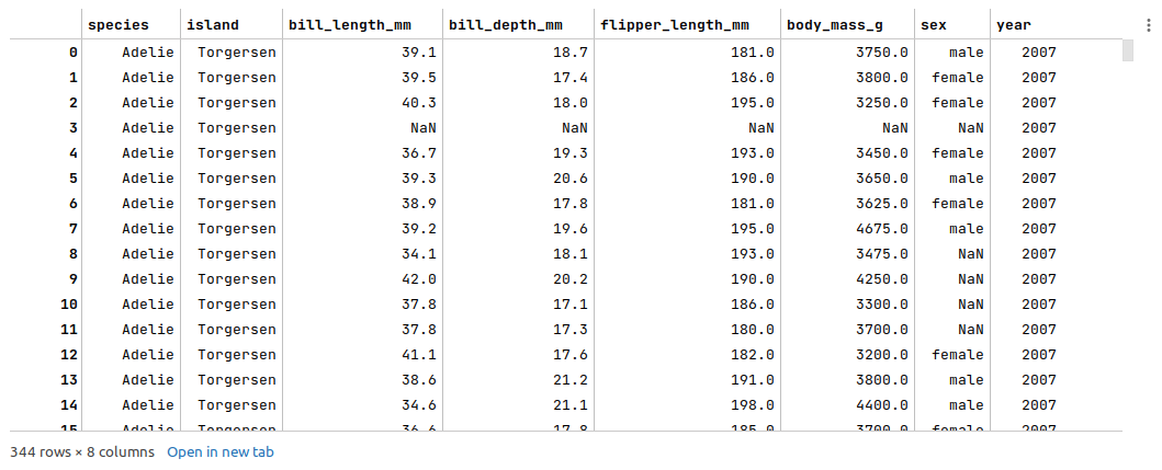
The next step is to load the palmer penguins data set into a pandas dataframe, drop the index column, and then display the dataframe as shown below:

url = 'https://vincentarelbundock.github.io/Rdatasets/csv/palmerpenguins/penguins.csv'
penguins_df = pd.read_csv(url)
penguins_df = penguins_df.drop(penguins_df.columns[0], axis=1)
penguins_df

The following illustration displays few rows from the palmer penguins dataframe:

The next step is to remediate the missing values from the palmer penguins dataframe. Note that we went through the steps to fix the missing values in the article Random Forest using Scikit-Learn, so we will not repeat it here.

For each of the missing values, we perform data analysis such as comparing the mean or (mean + std) values for the features and apply the following fixes as shown below:

penguins_df = penguins_df.drop([3, 271], axis=0)
penguins_df.loc[[8, 10, 11], 'sex'] = 'female'
penguins_df.at[9, 'sex'] = 'male'
penguins_df.at[47, 'sex'] = 'female'
penguins_df.loc[[178, 218, 256, 268], 'sex'] = 'female'

The next step is to display information about the palmer penguins dataframe, such as index and column types, memory usage, etc., as shown below:

The following illustration displays information about the palmer penguins dataframe:

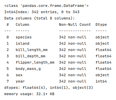
Note that there are no missing values at this point in the palmer penguins dataframe.

The next step is to create and display dummy binary variables for the two categorical (nominal) feature variables - island and sex from the cleansed palmer penguins dataframe as shown below:

nom_features = ['island', 'sex']
nom_encoded_df = pd.get_dummies(penguins_df[nom_features], prefix_sep='.', drop_first=True, sparse=False)
nom_encoded_df

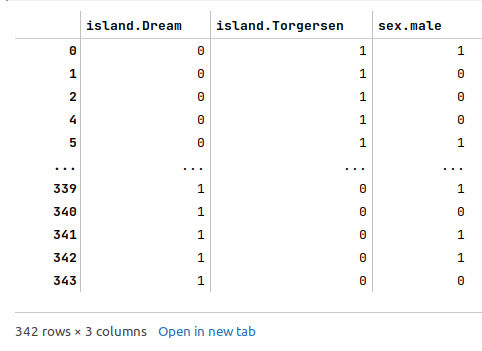
The following illustration displays the dataframe of all dummy binary variables for the two categorical (nominal) feature variables from the cleansed palmer penguins dataframe:

The next step is to drop the two nominal categorical features and merge the dataframe of dummy binary variables into the cleansed palmer penguins dataframe as shown below:

penguins_df2 = penguins_df.drop(penguins_df[nom_features], axis=1)
penguins_df3 = pd.concat([penguins_df2, nom_encoded_df], axis=1)
penguins_df3

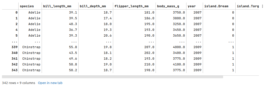
The following illustration displays few columns/rows from the merged palmer penguins dataframe:

The next step is to split the palmer penguins dataframe into two parts - a training data set and a test data set. The training data set is used to train the ensemble model and the test data set is used to evaluate the ensemble model. In this use case, we split 75% of the samples into the training dataset and remaining 25% into the test dataset as shown below:

X_train, X_test, y_train, y_test = train_test_split(penguins_df3, penguins_df3['species'], test_size=0.25, random_state=101)
X_train = X_train.drop('species', axis=1)
X_test = X_test.drop('species', axis=1)

The next step is to initialize the AdaBoost model class from scikit-learn and train the model using the training data set as shown below:

model = AdaBoostClassifier(n_estimators=100, learning_rate=0.01, random_state=101)
model.fit(X_train, y_train)

The following are a brief description of some of the hyperparameters used by the AdaBoost model:

n_estimators - the total number of trees in the ensemble. The default value is 50
learning_rate - controls the significance for each weak model (decision tree) in the ensemble. The default value is 1

The next step is to use the trained model to predict the species using the test dataset as shown below:

y_predict = model.predict(X_test)

The next step is to display the accuracy score for the model performance as shown below:

accuracy_score(y_test, y_predict)

The following illustration displays the accuracy score for the model performance:

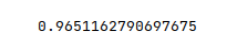
From the above, one can infer that the model seems to predict with accuracy.

The following is the link to the Jupyter Notebook that provides an hands-on demo for this article:

AdaBoost