Figure.1
| PolarSPARC |
Deep Learning - Gated Recurrent Unit
| Bhaskar S | 11/03/2023 |
Introduction
In the previous article Long Short Term Memory of this series, we provided an explanation of the inner workings of the LSTM model and how it mitigates the Vanishing Gradient issue.
In 2014, the Gated Recurrent Unit model (or GRU for short) was introduced as a more efficient alternative than the LSTM model.
Gated Recurrent Unit
GRU is a more recent model that does away with the long term memory (the Cell state) and using fewer parameters than the LSTM model, and yet with an ability to remember the longer term historical context.
One can basically think of the GRU model as an enhanced version of the RNN model that is not susceptible to the Vanishing Gradient problem.
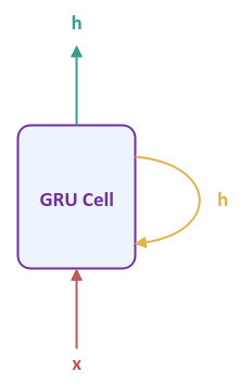
The following illustration shows the high-level abstraction of a Gated Recurrent Unit cell:
The output from the GRU model is the hidden state $h$ from the current time step, which also captures the long term context from the sequence of inputs that has been processed until the current time step. $x$ is the next input into the model.
Notice that the GRU Cell does not show any weight parameters and that is intentional as the computations in the GRU Cell are more complex than the RNN Cell.
The following illustration shows the Gated Recurrent Unit network unfolded over time for a sequence of $3$ inputs:
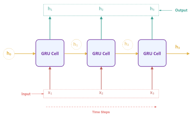
Notice that the unfolded network in Figure.2 above looks very similar to that of an RNN network. The difference is inside the GRU Cell.
Now, for the question on what magic happens inside the GRU Cell with the next input $x$ in the sequence and the previous value of the hidden state $h$ to generate the output ???
The following illustration depicts the computation graph inside the GRU Cell:
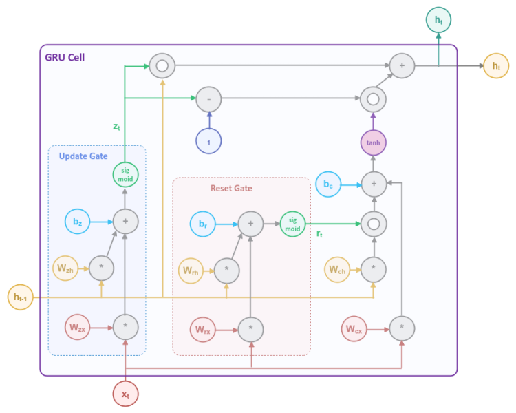
The computational graph may appear complicated, but in the following paragraphs, we will unpack and explain each of the blocks, so it becomes more clear.
The Reset Gate block in Figure.3 controls what percentage of the information from the previous hidden state needs to be forgotten.
The following illustration focuses on the Reset Gate block:
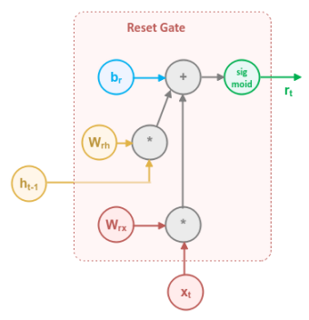
The Reset Gate uses the input $x_t$ from the current time step along with the output $h_{t-1}$ from the previous time step and applies the Sigmoid activation function to generate a numeric value between $0.0$ and $1.0$, which acts like the percentage knob to control how much information from the previous time step needs to be forgotten and what portion carried forward.
In mathematical terms, the computation that happen inside the first section of the Reset Gate is as follows:
$r_t = sigmoid(W_{rx} * x_t + W_{rh} * h_{t-1} + b_r)$
where $W_{rx}$ and $W_{rh}$ are the weights associated with the input $x_t$ and the previous output $h_{t-1}$ respectively, while $b_r$ is the bias.
The following illustration focuses on the section to the right of the Reset Gate block in Figure.3:
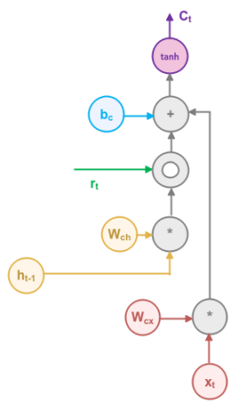
This section combines the output from the Reset Gate with the output $h_{t-1}$ from the previous time step using the element-wise (or hadamard) product and then adds it to the weighted input $x_t$ from the current time step. Finally, it applies the Tanh activation function to generate a numeric value between $-1.0$ and $1.0$, which determines how much of information from the Reset Gate $r_t$ and the input $x_t$ from the current time step, taken together, needs to be removed or added. In other words, the output from this section is the proposed candidate hidden state that is to be carried forward to the next time step.
In mathematical terms, the computation that happen inside this section is as follows:
$C_t = tanh(W_{cx} * x_t + r_t \odot h_{t-1} + b_c)$
where $\odot$ is the element-wise vector multiplication.
where $W_{cx}$ is the weight associated with the input $x_t$ and $b_c$ is the bias.
The Update Gate in Figure.3 above controls what percentage of the information from the previous hidden state and the candidate hidden state needs to be retained and passed along.
The following illustration focuses on the Update Gate block:
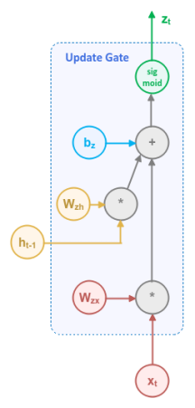
The Update Gate uses the input $x_t$ from the current time step along with the output $h_{t-1}$ from the previous time step and applies the Sigmoid activation function to generate a numeric value between $0.0$ and $1.0$, which acts like the percentage knob to control how much of information from the previous time step and the proposed hidden state needs to be retained and passed along to the next time step.
In mathematical terms, the computation that happen inside the Update Gate is as follows:
$z_t = sigmoid(W_{zx} * x_t + W_{zh} * h_{t-1} + b_z)$
where $W_{zx}$ and $W_{zh}$ are the weights associated with the input $x_t$ and the previous output $h_{t-1}$ respectively, while $b_z$ is the bias.
The following illustration focuses on the computation of the final hidden state, which will be passed to the next time step:
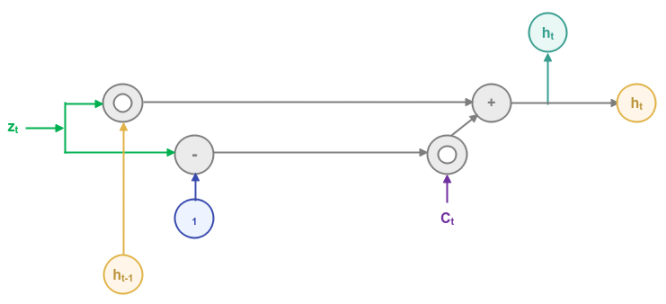
If the output $z_t$ from the Update Gate close to $1$, then a major portion of information from the previous time step is retained and information from the current time step is discarded (because of $1 - z_t$) and vice versa.
In other words, the output $z_t$ from the Update Gate acts like the percentage knob to control how much information from the previous and current time steps need to be carried forward.
In mathematical terms, the computation of the final hidden state $h_t$ for the current time step is as follows:
$h_t = z_t \odot h_{t-1} + (1 - z_t) \odot C_t$
where $\odot$ is the element-wise vector multiplication.
Hopefully the unpacking of each of the blocks helped clarify on what is going inside the GRU Cell.
Hands-on GRU Using PyTorch
We will demonstrate how one could leverage the GRU model for predicting the Next Word following a sequence using a toy corpus.
To predict the next word following a sequence of input words, we will train the LSTM model using the popular Aesop's Fable found here The Goose & the Golden Egg.
To import the necessary Python module(s), execute the following code snippet:
import numpy as np
import random
import torch
from nltk.tokenize import WordPunctTokenizer
from torch import nn
In order to ensure reproducibility, we need to set the seed to a constant value by executing the following code snippet:
seed_value = 101

torch.manual_seed(seed_value)
Copy the contents of the The Goose & the Golden Egg fable into a variable by executing the following code snippet:
corpus_text = '''There was once a Countryman who possessed the most wonderful Goose you can imagine, for every day when he visited the nest, the Goose had laid a beautiful, glittering, golden egg. The Countryman took the eggs to market and soon began to get rich. But
it was not long before he grew impatient with the Goose because she gave him only a single golden egg a day. He was not getting rich fast enough.
Then one day, after he had finished counting his money, the idea came to him that he could get all the golden eggs at once by killing the Goose and cutting it open. But when the deed was done, not a single golden egg did he find, and his precious Goose was dead.'''
To display the length of the corpus, execute the following code snippet:
len(corpus_text)
The following would be a typical output:
659
To define a function to extract all the word tokens from the corpus, execute the following code snippet:
def extract_corpus_words(corpus):
  word_tokenizer = WordPunctTokenizer()
  tokens = word_tokenizer.tokenize(corpus)
  all_tokens = [word.lower() for word in tokens if word.isalpha()]
  return all_tokens
To extract all the word tokens from the given corpus and display the first 10 words, execute the following code snippet:
corpus_tokens = extract_corpus_words(corpus_text)
corpus_tokens[:10]
The following would be a typical output:
['there',
 'was',
 'once',
 'a',
 'countryman',
 'who',
 'possessed',
 'the',
 'most',
 'wonderful']
To define a function to extract all the unique words (vocabulary) from the corpus, execute the following code snippet:
def extract_corpus_vocab(all_words):
  vocab_words = list(set(all_words))
  vocab_words.sort()
  return vocab_words
To extract all the unique words (vocabulary) from the given corpus and display the first 10 words, execute the following code snippet:
vocab_words_list = extract_corpus_vocab(corpus_tokens)
vocab_words_list[:10]
The following would be a typical output:
['a',
 'after',
 'all',
 'and',
 'at',
 'beautiful',
 'because',
 'before',
 'began',
 'but']
To display the number of unique words (vocabulary), execute the following code snippet:
len(vocab_words_list)
The following would be a typical output:
76
We know that neural network models only deal with numbers. To define a function to assign a numeric value to each of the unique words (vocabulary) from the corpus, execute the following code snippet:
def assign_word_number(words):
  words_index = {}
  for idx, word in enumerate(words):
    words_index[word] = idx
  return words_index
To assign a numeric value to each of the unique words (vocabulary) from the given corpus, execute the following code snippet:
word_to_nums = assign_word_number(vocab_words_list)
For our training set, we will consider 3-grams, meaning a sequence of three words from the corpus. To define a function to generate the training set of 3-grams from the corpus, execute the following code snippet:
ngram_size = 3

def create_ngram_sequences(tokens):
  ngrams_list = []
  for i in range(ngram_size, len(tokens) + 1):
    ngrams = tokens[i - ngram_size:i]
    ngrams_list.append(ngrams)
  return ngrams_list
To generate the training set of 3-grams from the corpus and display the first 10 sequences, execute the following code snippet:
ngram_sequences = create_ngram_sequences(corpus_tokens)
ngram_sequences[:10]
The following would be a typical output:
[['there', 'was', 'once'],
 ['was', 'once', 'a'],
 ['once', 'a', 'countryman'],
 ['a', 'countryman', 'who'],
 ['countryman', 'who', 'possessed'],
 ['who', 'possessed', 'the'],
 ['possessed', 'the', 'most'],
 ['the', 'most', 'wonderful'],
 ['most', 'wonderful', 'goose'],
 ['wonderful', 'goose', 'you']]
To display the number of training sequences, execute the following code snippet:
len(ngram_sequences)
The following would be a typical output:
125
To define a function to convert the sequence of words to the sequence of their corresponding assigned numeric values, execute the following code snippet:
def ngram_sequences_to_numbers(seq_list):
  ngram_numbers_list = []
  for ngrams in seq_list:
    num_seq = []
    for word in ngrams:
      num_seq.append(word_to_nums.get(word))
    ngram_numbers_list.append(num_seq)
  return ngram_numbers_list
To convert the sequence of words from the training set to the corresponding sequence of numbers and display the first 10 set of numerical sequences, execute the following code snippet:
ngram_seq_nums = ngram_sequences_to_numbers(ngram_sequences)
ngram_seq_nums[:10]
The following would be a typical output:
[[66, 70, 53],
 [70, 53, 0],
 [53, 0, 15],
 [0, 15, 72],
 [15, 72, 57],
 [72, 57, 64],
 [57, 64, 50],
 [64, 50, 74],
 [50, 74, 35],
 [74, 35, 75]]
For training the neural network model, one should do so on a GPU device for efficiency. To select the GPU device if available, execute the following code snippet:
device = 'cuda' if torch.cuda.is_available() else 'cpu'
To create a tensor object from the numeric sequences and display the first 10 items, execute the following code snippet:
ngram_nums = torch.tensor(ngram_seq_nums, device=device)
ngram_nums[:10]
The following would be a typical output:
tensor([[66, 70, 53],
       [70, 53,  0],
       [53,  0, 15],
       [ 0, 15, 72],
       [15, 72, 57],
       [72, 57, 64],
       [57, 64, 50],
       [64, 50, 74],
       [50, 74, 35],
       [74, 35, 75]], device='cuda:0')
To create the feature and target tensors from the training set, execute the following code snippet:
X_train = ngram_nums[:, :-1]
y_target = ngram_nums[:, -1]
To define a function to convert the target numeric values to one-hot representation, execute the following code snippet:
one_hot_size = len(vocab_words_list)

def word_num_to_onehot(target):
  one_hot_list = []
  for idx in target:
    one_hot = np.zeros(one_hot_size, dtype=np.float32)
    one_hot[idx] = 1.0
    one_hot_list.append(one_hot)
  return one_hot_list
To convert the target tensor object to equivaled one-hot representation and display the first 5 items, execute the following code snippet:
y_one_hot = word_num_to_onehot(y_target)
y_one_hot_target = torch.tensor(np.asarray(y_one_hot), device=device)
y_one_hot_target[:5]
The following would be a typical output:
tensor([[0., 0., 0., 0., 0., 0., 0., 0., 0., 0., 0., 0., 0., 0., 0., 0., 0., 0.,
         0., 0., 0., 0., 0., 0., 0., 0., 0., 0., 0., 0., 0., 0., 0., 0., 0., 0.,
         0., 0., 0., 0., 0., 0., 0., 0., 0., 0., 0., 0., 0., 0., 0., 0., 0., 1.,
         0., 0., 0., 0., 0., 0., 0., 0., 0., 0., 0., 0., 0., 0., 0., 0., 0., 0.,
         0., 0., 0., 0.],
        [1., 0., 0., 0., 0., 0., 0., 0., 0., 0., 0., 0., 0., 0., 0., 0., 0., 0.,
         0., 0., 0., 0., 0., 0., 0., 0., 0., 0., 0., 0., 0., 0., 0., 0., 0., 0.,
         0., 0., 0., 0., 0., 0., 0., 0., 0., 0., 0., 0., 0., 0., 0., 0., 0., 0.,
         0., 0., 0., 0., 0., 0., 0., 0., 0., 0., 0., 0., 0., 0., 0., 0., 0., 0.,
         0., 0., 0., 0.],
        [0., 0., 0., 0., 0., 0., 0., 0., 0., 0., 0., 0., 0., 0., 0., 1., 0., 0.,
         0., 0., 0., 0., 0., 0., 0., 0., 0., 0., 0., 0., 0., 0., 0., 0., 0., 0.,
         0., 0., 0., 0., 0., 0., 0., 0., 0., 0., 0., 0., 0., 0., 0., 0., 0., 0.,
         0., 0., 0., 0., 0., 0., 0., 0., 0., 0., 0., 0., 0., 0., 0., 0., 0., 0.,
         0., 0., 0., 0.],
        [0., 0., 0., 0., 0., 0., 0., 0., 0., 0., 0., 0., 0., 0., 0., 0., 0., 0.,
         0., 0., 0., 0., 0., 0., 0., 0., 0., 0., 0., 0., 0., 0., 0., 0., 0., 0.,
         0., 0., 0., 0., 0., 0., 0., 0., 0., 0., 0., 0., 0., 0., 0., 0., 0., 0.,
         0., 0., 0., 0., 0., 0., 0., 0., 0., 0., 0., 0., 0., 0., 0., 0., 0., 0.,
         1., 0., 0., 0.],
        [0., 0., 0., 0., 0., 0., 0., 0., 0., 0., 0., 0., 0., 0., 0., 0., 0., 0.,
         0., 0., 0., 0., 0., 0., 0., 0., 0., 0., 0., 0., 0., 0., 0., 0., 0., 0.,
         0., 0., 0., 0., 0., 0., 0., 0., 0., 0., 0., 0., 0., 0., 0., 0., 0., 0.,
         0., 0., 0., 1., 0., 0., 0., 0., 0., 0., 0., 0., 0., 0., 0., 0., 0., 0.,
         0., 0., 0., 0.]], device='cuda:0')
To create the GRU model to predict the next word given a sequence of two input words, execute the following code snippet:
num_features = X_train.shape[1]
vocab_size = one_hot_size
embed_size = 128
hidden_size = 128
output_size = one_hot_size
dropout_rate = 0.2

class NextWordGRU(nn.Module):
  def __init__(self, vocab_sz, embed_sz, hidden_sz, output_sz):
    super(NextWordGRU, self).__init__()
    self.embed = nn.Embedding(vocab_sz, embed_sz)
    self.lstm = nn.GRU(input_size=embed_sz, hidden_size=hidden_sz)
    self.dropout = nn.Dropout(dropout_rate)
    self.linear = nn.Linear(hidden_size*num_features, output_sz)

  def forward(self, x_in: torch.Tensor):
    embedded = self.embed(x_in)
    output, _ = self.lstm(embedded)
    output = output.view(output.size(0), -1)
    output = self.dropout(output)
    output = self.linear(output)
    return output
To create an instance of the NextWordGRU model, execute the following code snippet:
nw_model = NextWordGRU(vocab_size, embed_size, hidden_size, output_size)
nw_model.to(device)
Since the next word can be anyone from the vocabulary, we will create an instance of the Cross Entropy loss function by executing the following code snippet:
criterion = nn.CrossEntropyLoss()
criterion.to(device)
To create an instance of the gradient descent function, execute the following code snippet:
learning_rate = 0.01

optimizer = torch.optim.Adam(nw_model.parameters(), lr=learning_rate)
To implement the iterative training loop for the forward pass to predict, compute the loss, and execute the backward pass to adjust the parameters, execute the following code snippet:
num_epochs = 51

for epoch in range(1, num_epochs):
  nw_model.train()
  optimizer.zero_grad()
  y_predict = nw_model(X_train)
  loss = criterion(y_predict, y_one_hot_target)
  if epoch % 5 == 0:
    print(f'Next Word Model GRU -> Epoch: {epoch}, Loss: {loss}')
  loss.backward()
  optimizer.step()
The following would be a typical output:
Next Word Model GRU -> Epoch: 5, Loss: 1.2131516933441162
Next Word Model GRU -> Epoch: 10, Loss: 0.0475066713988781
Next Word Model GRU -> Epoch: 15, Loss: 0.006809725426137447
Next Word Model GRU -> Epoch: 20, Loss: 0.001894962857477367
Next Word Model GRU -> Epoch: 25, Loss: 0.0005625554476864636
Next Word Model GRU -> Epoch: 30, Loss: 0.0005398059147410095
Next Word Model GRU -> Epoch: 35, Loss: 0.0002399681106908247
Next Word Model GRU -> Epoch: 40, Loss: 0.00017658475553616881
Next Word Model GRU -> Epoch: 45, Loss: 0.00018268678104504943
Next Word Model GRU -> Epoch: 50, Loss: 0.00012366866576485336
Given that we have completed the model training, we can bring the model back to the CPU device by executing the following code snippet:
device_cpu = 'cpu'

nw_model.to(device_cpu)
To define a function to randomly pick a sequence from the training set, execute the following code snippet:
def pick_ngram_sub_sequence(seq_list):
  idx = random.randint(0, len(seq_list))
  return seq_list[idx], seq_list[idx][:-1]
To evaluate the trained model, we will run about $10$ trials. In each trial, we randomly pick a word sequence, convert the selected word sequence to numeric sequence, create a tensor object for the converted numeric sequence, and then predict the next word for the selected numeric sequence. To run the trials, execute the following code snippet:
num_trials = 10

for i in range(1, num_trials+1):
  ngram_seq_pick, ngram_sub_seq = pick_ngram_sub_sequence(ngram_sequences)
  print(f'Trial #{i} - Picked sequence: {ngram_seq_pick}, Test sub-sequence: {ngram_sub_seq}')
  ngram_sub_seq_num = ngram_sequences_to_numbers([ngram_sub_seq])
  X_test = torch.tensor(ngram_sub_seq_num)
  print(f'Trial #{i} - X_test: {X_test}')
  nw_model.eval()
  with torch.no_grad():
    y_predict = nw_model(X_test)
    idx = torch.argmax(y_predict)
    print(f'Trial #{i} - idx: {idx}, next word: {vocab_words_list[idx]}')
The following would be a typical output:
Trial #1 - Picked sequence: ['rich', 'fast', 'enough'], Test sub-sequence: ['rich', 'fast']
Trial #1 - X_test: tensor([[59, 26]])
Trial #1 - idx: 24, next word: enough
Trial #2 - Picked sequence: ['long', 'before', 'he'], Test sub-sequence: ['long', 'before']
Trial #2 - X_test: tensor([[47,  7]])
Trial #2 - idx: 38, next word: he
Trial #3 - Picked sequence: ['day', 'when', 'he'], Test sub-sequence: ['day', 'when']
Trial #3 - X_test: tensor([[17, 71]])
Trial #3 - idx: 38, next word: he
Trial #4 - Picked sequence: ['it', 'open', 'but'], Test sub-sequence: ['it', 'open']
Trial #4 - X_test: tensor([[44, 56]])
Trial #4 - idx: 9, next word: but
Trial #5 - Picked sequence: ['to', 'him', 'that'], Test sub-sequence: ['to', 'him']
Trial #5 - X_test: tensor([[67, 39]])
Trial #5 - idx: 63, next word: that
Trial #6 - Picked sequence: ['began', 'to', 'get'], Test sub-sequence: ['began', 'to']
Trial #6 - X_test: tensor([[ 8, 67]])
Trial #6 - idx: 31, next word: get
Trial #7 - Picked sequence: ['there', 'was', 'once'], Test sub-sequence: ['there', 'was']
Trial #7 - X_test: tensor([[66, 70]])
Trial #7 - idx: 53, next word: once
Trial #8 - Picked sequence: ['to', 'market', 'and'], Test sub-sequence: ['to', 'market']
Trial #8 - X_test: tensor([[67, 48]])
Trial #8 - idx: 3, next word: and
Trial #9 - Picked sequence: ['did', 'he', 'find'], Test sub-sequence: ['did', 'he']
Trial #9 - X_test: tensor([[20, 38]])
Trial #9 - idx: 27, next word: find
Trial #10 - Picked sequence: ['for', 'every', 'day'], Test sub-sequence: ['for', 'every']
Trial #10 - X_test: tensor([[29, 25]])
Trial #10 - idx: 17, next word: day
WOW !!! As can be inferred from the Output.11 above, the success rate is $100\%$.
References