Figure.1
| PolarSPARC |
Deep Learning - Long Short Term Memory
| Bhaskar S | 08/25/2023 |
Introduction
In the previous article Recurrent Neural Network of this series, we provided an explanation of the inner workings and a practical demo of RNN for the restaurant reviews sentiment prediction.
For a long sequence of text input, the RNN model tends to forget the text context from earlier on due to the Vanishing Gradient problem, resulting in a poor prediction performance.
To address the long term memory retention in RNN is where the Long Short Term Memory (or LSTM for short) comes into play.
Long Short Term Memory
LSTM is basically an enhanced version of RNN with an additional memory state to remember longer term historical context.
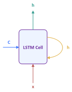
The following illustration shows the high-level abstraction of a Long Short Term Memory cell:
The output from the LSTM model is the hidden state $h$ for the current time step. $x$ is the next input into the model. The parameter $C$ is the cell state which captures the long term context from the sequence of inputs that has been processed until the current time step.
Notice that the LSTM Cell does not show any weight parameters and that is intentional as the computations in the LSTM Cell are more complex than the RNN Cell.
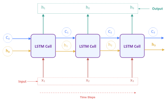
The following illustration shows the Long Short Term Memory network unfolded over time for a sequence of $3$ inputs:
Now, for the question on what magic happens inside the LSTM Cell with the next input $x$ in the sequence, the previous value of the cell state $C$, and the previous value of the hidden state $h$ to generate the output ???
The following illustration depicts the computation graph inside the LSTM Cell:
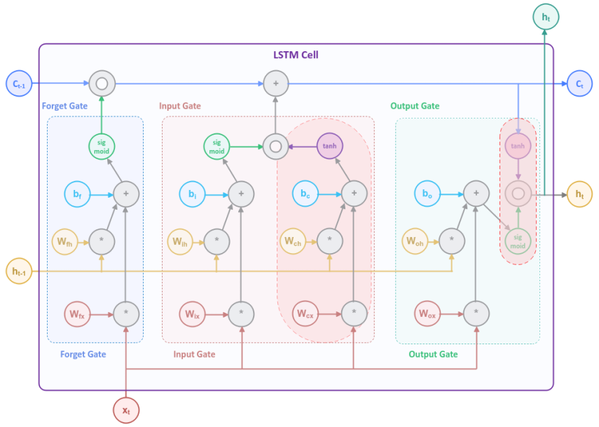
Looks complicated and SCARY ??? Don't sweat it - RELAX !!! In the following paragraphs, we will unpack each of the blocks and explain, so it becomes more clear.
The first block in Figure.3 above is referred to as the Forget Gate and controls what percentage of the information from the cell state (long term memory) needs to be forgotten or remembered.
The following illustration focuses on the Forget Gate block:
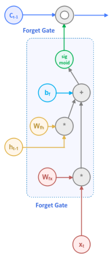
The Forget Gate uses the input $x_t$ from the current time step along with the output $h_{t-1}$ from the previous time step and applies the Sigmoid activation function to generate a numeric value between $0.0$ and $1.0$, which acts like the percentage knob to control the retention in the long term memory from the current time step.
In mathematical terms, the computation that happen inside the Forget Gate is as follows:
$f_t = sigmoid(W_{fx} * x_t + W_{fh} * h_{t-1} + b_f)$
where $W_{fx}$ and $W_{fh}$ are the weights associated with the input $x_t$ and the previous output $h_{t-1}$ respectively, while $b_f$ is the bias.
The next block in Figure.3 above is referred to as the Input Gate and controls what percentage of the information from the current input needs to be preserved and stored in the cell state (long term memory) along with the cell state from the previous time step.
The following illustration focuses on first section of the Input Gate block, with the second section greyed out:
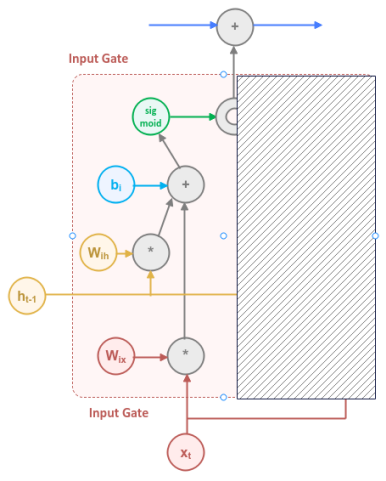
The first section of the Input Gate uses the input $x_t$ from the current time step along with the output $h_{t-1}$ from the previous time step and applies the Sigmoid activation function to generate a numeric value between $0.0$ and $1.0$, which acts like the percentage knob to control how much information from the current time step needs to be retained.
In mathematical terms, the computation that happen inside the first section of the Input Gate is as follows:
$i_t = sigmoid(W_{ix} * x_t + W_{ih} * h_{t-1} + b_i)$
where $W_{ix}$ and $W_{ih}$ are the weights associated with the input $x_t$ and the previous output $h_{t-1}$ respectively, while $b_i$ is the bias.
The following illustration focuses on second section of the Input Gate block, with the first section greyed out:
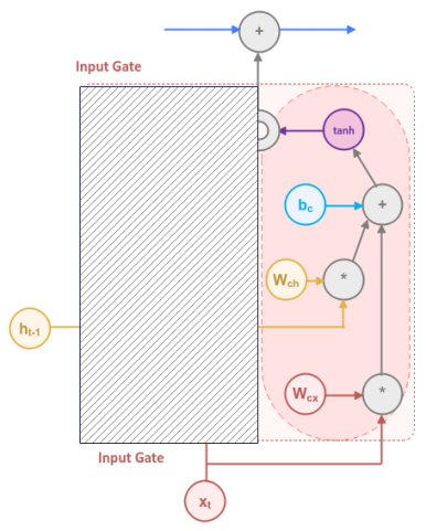
The second section of the Input Gate is creating a cell state from the input $x_t$ in the current time step along with the output $h_{t-1}$ from the previous time step and applies the Tanh activation function to generate a numeric value between $-1.0$ and $1.0$, which determines how much of the information from the current time step to remove or add from the next cell state.
In mathematical terms, the computation that happen inside the second section of the Input Gate is as follows:
$\tilde{c_t} = tanh(W_{cx} * x_t + W_{ch} * h_{t-1} + b_c)$
where $W_{cx}$ and $W_{ch}$ are the weights associated with the input $x_t$ and the previous output $h_{t-1}$ respectively, while $b_c$ is the bias.
The following illustration focuses on the outputs from the Forget Gate and Input Gate blocks:
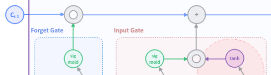
The outputs from the Forget Gate and Input Gate blocks are used along with the cell state $c_{t-1}$ from the previous time step to generate the next cell state $c_t$.
In mathematical terms, the computation that happens to update the next cell state $c_t$ is as follows:
$c_t = c_{t-1} \odot f_t + i_t \odot \tilde{c_t}$
where $\odot$ is the element-wise vector multiplication.
Given that there is NO weight or bias involved in the computation of $c_t$, it is NOT effected by the Vanishing Gradient problem.
The final block in Figure.3 above is referred to as the Output Gate and determines the next output based on the current adjusted cell state $c_t$ (long term memory) along with the previous hidden state $h_{t-1}$ (short term memory).
The following illustration focuses on first section of the Output Gate block, with the second section greyed out:
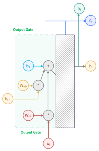
The first section of the Output Gate uses the input $x_t$ from the current time step along with the output $h_{t-1}$ from the previous time step and applies the Sigmoid activation function to generate a numeric value between $0.0$ and $1.0$, which acts like the percentage knob to control how much information from the current time step needs to be retained in the next output.
In mathematical terms, the computation that happen inside the first section of the Output Gate is as follows:
$o_t = sigmoid(W_{ox} * x_t + W_{oh} * h_{t-1} + b_o)$
where $W_{ox}$ and $W_{oh}$ are the weights associated with the input $x_t$ and the previous output $h_{t-1}$ respectively, while $b_o$ is the bias.
The following illustration focuses on the second section of the Output Gate block:
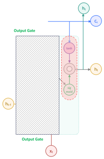
The output from the Output Gate block is consumed along with the current computed cell state $c_t$ to generate the next hidden state $h_t$, which also happens to be the output.
In mathematical terms, the computation that happens to update the next hidden state $h_t$ is as follows:
$h_t = o_t \odot tanh(c_t)$
where $\odot$ is the element-wise vector multiplication.
PHEW !!! Hopefully the unpacking of each of the blocks helped clarify on what is going inside the LSTM Cell.
Dropout Regularization
When training neural network models with lots of hidden layers using a small training dataset, the model generally tends to OVERFIT. As a result, the trained neural network model performs poorly during evaluation.
One way to deal with overfitting would be to train an ENSEMBLE of neural network models and take their average. For very large neural network models, this approach is not always practical due to resource and time constraints.
This is where the concept of Dropout comes in handy, which performs corrections by randomly "dropping" (or disabling) some nodes from an input layer and/or a hidden layer temporarily. This behavior has the same "effect" as running an ensemble model.
To perform the Dropout Regularization, one must specify a "dropout" rate, which typically is a value between $0.2$ and $0.5$.
Hands-on LSTM Using PyTorch
To perform sentiment analysis using the LSTM model, we will be leveraging the Restaurant Reviews data set from Kaggle.
To import the necessary Python module(s), execute the following code snippet:
import numpy as np
import pandas as pd
import nltk
import torch
from collections import Counter
from nltk.corpus import stopwords
from nltk.tokenize import WordPunctTokenizer
from sklearn.model_selection import train_test_split
from torch import nn
from torchmetrics import Accuracy
Assuming the logged in user is alice, to set the correct path to the nltk data packages, execute the following code snippet:
nltk.data.path.append("/home/alice/nltk_data")
Download the Kaggle Restaurant Reviews data set to the directory /home/alice/txt_data.
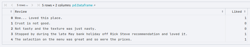
To load the tab-separated restaurant reviews data set into pandas and display the first few rows, execute the following code snippet:
reviews_df = pd.read_csv('./txt_data/Restaurant_Reviews.tsv', sep='\t')
reviews_df.head()
The following would be a typical output:
To create an instance of the stop words, the word tokenizer, and the lemmatizer, execute the following code snippet:
stop_words = stopwords.words('english')
word_tokenizer = WordPunctTokenizer()
word_lemmatizer = nltk.WordNetLemmatizer()
To extract all the text reviews as a list of sentences (corpus), execute the following code snippet:
reviews_txt = reviews_df.Review.values.tolist()
To cleanse the sentences from the corpus by removing the punctuations, stop words, two-letter words, converting words to their roots, collecting all the unique words from the reviews corpus, execute the following code snippet:
vocabulary_counter = Counter()
cleansed_review_txt = []
for review in reviews_txt:
  tokens = word_tokenizer.tokenize(review)
  alpha_words = [word.lower() for word in tokens if word.isalpha() and len(word) > 2 and word not in stop_words]
  final_words = [word_lemmatizer.lemmatize(word) for word in alpha_words]
  vocabulary_counter.update(final_words)
  cleansed_review = ' '.join(final_words)
  cleansed_review_txt.append(cleansed_review)
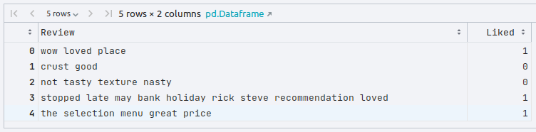
To update the original reviews in the reviews pandas dataframe with the cleansed restaurant reviews display the first few rows, execute the following code snippet:
reviews_df['Review'] = cleansed_review_txt
reviews_df.head()
The following would be a typical output:
We need an index position for each word in the corpus. For this demonstration, we will use $500$ of the most common words. To create a word to index dictionary for the most common words, execute the following code snippet:
one_hot_size = 500
common_vocabulary = vocabulary_counter.most_common(one_hot_size)
word_to_index = {word:idx for idx, (word, count) in enumerate(common_vocabulary)}
We will use the word to index dictionary from above to convert each of the restaurant reviews (in text form) to a one-hot encoded vector (of numbers - ones for word present or zeros for absent). To create a list of one-hot encoded vector for each of the reviews, execute the following code snippet:
clean_reviews_txt = reviews_df.Review.values.tolist()
clean_reviews_labels = reviews_df.Liked.values.tolist()
one_hot_reviews_list = []
for review in clean_reviews_txt:
  tokens = word_tokenizer.tokenize(review)
  one_hot_review = np.zeros((one_hot_size), dtype=np.float32)
  for word in tokens:
    if word in word_to_index:
      one_hot_review[word_to_index[word]] = 1
  one_hot_reviews_list.append(one_hot_review)
To create the tensor objects for the input and the corresponding labels, execute the following code snippet:
X = torch.tensor(np.array(one_hot_reviews_list), dtype=torch.float)
y = torch.tensor(np.array(clean_reviews_labels), dtype=torch.float).unsqueeze(dim=1)
To create the training and testing data sets, execute the following code snippet:
X_train, X_test, y_train, y_test = train_test_split(X, y, test_size=0.2, random_state=101)
To initialize variables for the number of input features, the size of both the cell state and the hidden state, and the number of outputs, execute the following code snippet:
input_size = one_hot_size
hidden_size = 128
no_layers = 1
output_size = 1
To create an LSTM model for the reviews sentiment analysis using a single hidden layer, execute the following code snippet:
class SentimentLSTM(nn.Module):
  def __init__(self, input_sz, hidden_sz, output_sz):
    super(SentimentLSTM, self).__init__()
    self.lstm = nn.LSTM(input_size=input_sz, hidden_size=hidden_sz, num_layers=no_layers)
    self.linear = nn.Linear(hidden_size, output_sz)
    self.dropout = nn.Dropout(0.2)

  def forward(self, x_in: torch.Tensor):
    output, _ = self.lstm(x_in)
    output = self.linear(output)
    output = self.dropout(output)
    return output
To create an instance of the SentimentLSTM model, execute the following code snippet:
snt_model = SentimentLSTM(input_size, hidden_size, output_size)
Since the sentiments can either be positive or negative (binary), we will create an instance of the Binary Cross Entropy loss function by executing the following code snippet:
criterion = nn.BCEWithLogitsLoss()
Note that the BCEWithLogitsLoss loss function combines both the sigmoid activation function and the binary cross entropy loss function into a single function.
To create an instance of the gradient descent function, execute the following code snippet:
optimizer = torch.optim.SGD(snt_model.parameters(), lr=0.05)
To implement the iterative training loop for the forward pass to predict, compute the loss, and execute the backward pass to adjust the parameters, execute the following code snippet:
num_epochs = 5001
for epoch in range(1, num_epochs):
  snt_model.train()
  optimizer.zero_grad()
  y_predict = snt_model(X_train)
  loss = criterion(y_predict, y_train)
  if epoch % 500 == 0:
    print(f'Sentiment Model LSTM -> Epoch: {epoch}, Loss: {loss}')
  loss.backward()
  optimizer.step()
The following would be a typical output:
Sentiment Model LSTM -> Epoch: 500, Loss: 0.6887498497962952
Sentiment Model LSTM -> Epoch: 1000, Loss: 0.6818993091583252
Sentiment Model LSTM -> Epoch: 1500, Loss: 0.6695456504821777
Sentiment Model LSTM -> Epoch: 2000, Loss: 0.6460920572280884
Sentiment Model LSTM -> Epoch: 2500, Loss: 0.6167201995849609
Sentiment Model LSTM -> Epoch: 3000, Loss: 0.5674394965171814
Sentiment Model LSTM -> Epoch: 3500, Loss: 0.5004092454910278
Sentiment Model LSTM -> Epoch: 4000, Loss: 0.4361661672592163
Sentiment Model LSTM -> Epoch: 4500, Loss: 0.36369624733924866
Sentiment Model LSTM -> Epoch: 5000, Loss: 0.29472610354423523
To predict the target values using the trained model, execute the following code snippet:
snt_model.eval()
with torch.no_grad():
  y_predict = snt_model(X_test)
  y_predict = torch.round(y_predict)
To display the model prediction accuracy, execute the following code snippet:
accuracy = Accuracy(task='binary', num_classes=2)

print(f'Sentiment Model LSTM -> Accuracy: {accuracy(y_predict, y_test)}')
The following would be a typical output:
Sentiment Model LSTM -> Accuracy: 0.7699999809265137
This concludes the explanation and demonstration of a Long Short Term Memory model.
References
Deep Learning - Recurrent Neural Network
Deep Learning - The Vanishing Gradient
Introduction to Deep Learning - Part 7
Introduction to Deep Learning - Part 6
Introduction to Deep Learning - Part 5
Introduction to Deep Learning - Part 4
Introduction to Deep Learning - Part 3