Figure.1
| PolarSPARC |
Deep Learning - Recurrent Neural Network
| Bhaskar S | 08/13/2023 |
Introduction
There are use-cases in the natural language processing domain, such as, predicting the next word in a sentence, or predicting the sentiment of a sentence, etc. For these cases, notice that the size of the input is varying and more importantly the order of the words is crucial. Hence, the regular neural network would not work for these cases.
To process a variable number of ordered sequence of data, we need a different type of neural network and this is where the Recurrent Neural Network (or RNN for short) comes in handy.
Recurrent Neural Network
RNN is a neural network that processes a sequence of inputs $x_1, x_2, x_3,...,x_{t-1}, x_t$ at each time step to produce some output.
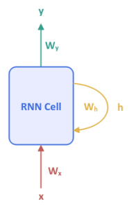
The following illustration shows the high-level abstraction of a Recurrent Neural Network:
$y$ is the output from the RNN model with $W_y$ as its weight parameter. $x$ is the next input into the model with $W_x$ as its weight parameter. The parameter $h$ is the hidden state which captures the historical sequence of inputs that has been processed until the current time step with $W_h$ as its weight parameter. One can think of $h$ as the memory of the neural network model.
The basic RNN model consists of a single hidden layer and the whole network is encapsulated into a single unit, which often referred to as an RNN Cell.
Notice that the RNN Cell is also fed the hidden state in addition to the input. This may seem a bit confusing and hence better visualized when the model is unfolded for the entire input sequence.
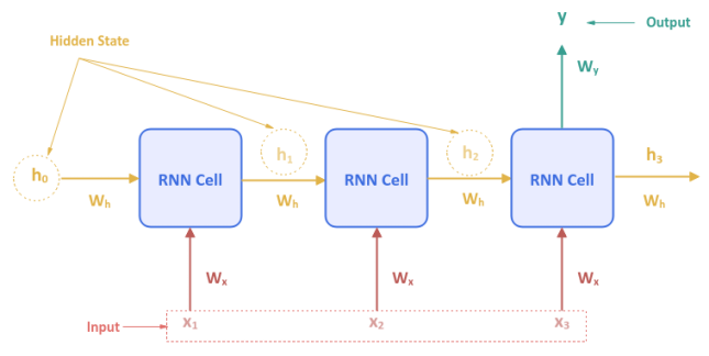
The following illustration shows the Recurrent Neural Network unfolded over time for a sequence of $3$ inputs:
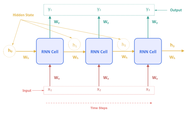
The initial hidden state $h_0$ at the first time step is set to ZERO. At the second time step, the hidden state $h_1$ from the previous time step is used along with the input $x_2$ and so on. This pattern repeats itself for the entire input sequence. Hence, the word Recurrent to indicate the pattern occurs repeatedly.
Notice that the weight parameters $W_x$, $W_h$, and $W_y$ are the same for each time step of the neural network model.
Now, for the question on what magic happens inside the RNN Cell with the next input $x$ in the sequence and the previous value of the hidden state $h$ to generate the output $y$ ???
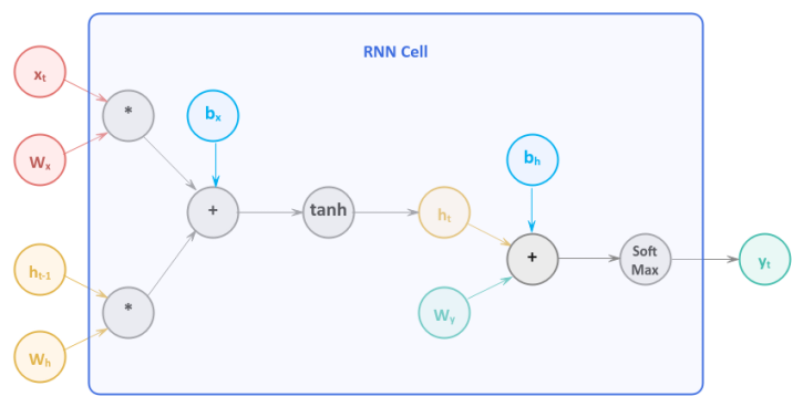
Two activation functions are used inside the RNN Cell - the first is the Hyperbolic Tan (or tanh) function and the second is the Softmax function.
With that, let us unravel the mathematical computations that happen inside the RNN Cell:
$h_t = tan(x_t * W_x + h_{t-1} * W_h + b_x)$
$y_t = softmax(h_t * W_y + b_h)$
where $t$ is the current time step, $t-1$ is the previous time step, $b_x$ is the bias for the input, and $b_h$ is the bias for the hidden state.
The following illustration depicts the computation graph inside the RNN Cell:
The RNN Cell we discussed above is referred to as the One-to-One network model. In other words, for each input there is one output. This type of a model can be used for the Image Classification use-case.
The following illustration depicts a One-to-Many RNN network model:
In the One-to-Many RNN network model, for each input there are more than one output. This type of a model can be used for the Image Captioning use-case.
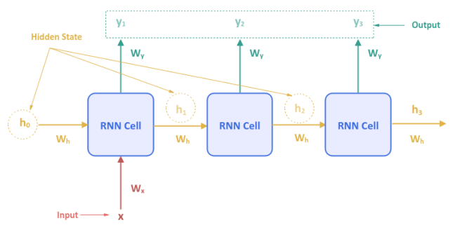
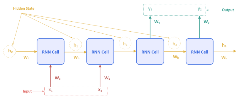
The following illustration depicts a Many-to-One RNN network model:
In the Many-to-One RNN network model, for a sequence of inputs there is one output. This type of a model can be used for the Sentiment Classification use-case.
The following illustration depicts a Many-to-Many RNN network model:
In the Many-to-Many RNN network model, for a sequence of inputs there are more than one output. This type of a model can be used for the Language Translation use-case.
As indicated in the very beginning, the basic RNN network model uses a single hidden layer. There is nothing preventing one from stacking an RNN Cell on top of one another to create multiple hidden layers.
The following illustration depicts an RNN network model with two hidden layer s:
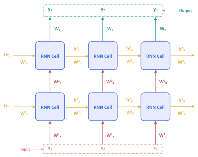
Note that the hidden state $h^1_t$ is associated with the first layer, $h^2_t$ with the second layer and so on.
For a long sequence of inputs, the Recurrent Neural Network model is susceptible to the dreaded Vanishing Gradient problem since the unfolding results in a deep network.
Hands-on RNN Using PyTorch
To perform sentiment analysis using the RNN model, we will be leveraging the Restaurant Reviews data set from Kaggle.
To import the necessary Python module(s), execute the following code snippet:
import numpy as np
import pandas as pd
import nltk
import torch
from collections import Counter
from nltk.corpus import stopwords
from nltk.tokenize import WordPunctTokenizer
from sklearn.model_selection import train_test_split
from torch import nn
from torchmetrics import Accuracy
Assuming the logged in user is alice, to set the correct path to the nltk data packages, execute the following code snippet:
nltk.data.path.append("/home/alice/nltk_data")
Download the Kaggle Restaurant Reviews data set to the directory /home/alice/txt_data.
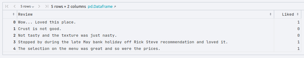
To load the tab-separated restaurant reviews data set into pandas and display the first few rows, execute the following code snippet:
reviews_df = pd.read_csv('./txt_data/Restaurant_Reviews.tsv', sep='\t')
reviews_df.head()
The following would be a typical output:
To create an instance of the stop words, the word tokenizer, and the lemmatizer, execute the following code snippet:
stop_words = stopwords.words('english')
word_tokenizer = WordPunctTokenizer()
word_lemmatizer = nltk.WordNetLemmatizer()
To extract all the text reviews as a list of sentences (corpus), execute the following code snippet:
reviews_txt = reviews_df.Review.values.tolist()
To cleanse the sentences from the corpus by removing the punctuations, stop words, two-letter words, converting words to their roots, collecting all the unique words from the reviews corpus, execute the following code snippet:
vocabulary_counter = Counter()
cleansed_review_txt = []
for review in reviews_txt:
  tokens = word_tokenizer.tokenize(review)
  alpha_words = [word.lower() for word in tokens if word.isalpha() and len(word) > 2 and word not in stop_words]
  final_words = [word_lemmatizer.lemmatize(word) for word in alpha_words]
  vocabulary_counter.update(final_words)
  cleansed_review = ' '.join(final_words)
  cleansed_review_txt.append(cleansed_review)
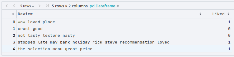
To update the original reviews in the reviews pandas dataframe with the cleansed restaurant reviews display the first few rows, execute the following code snippet:
reviews_df['Review'] = cleansed_review_txt
reviews_df.head()
The following would be a typical output:
We need an index position for each word in the corpus. For this demonstration, we will use $500$ of the most common words. To create a word to index dictionary for the most common words, execute the following code snippet:
one_hot_size = 500
common_vocabulary = vocabulary_counter.most_common(one_hot_size)
word_to_index = {word:idx for idx, (word, count) in enumerate(common_vocabulary)}
We will use the word to index dictionary from above to convert each of the restaurant reviews (in text form) to a one-hot encoded vector (of numbers - ones for word present or zeros for absent). To create a list of one-hot encoded vector for each of the reviews, execute the following code snippet:
clean_reviews_txt = reviews_df.Review.values.tolist()
clean_reviews_labels = reviews_df.Liked.values.tolist()
one_hot_reviews_list = []
for review in clean_reviews_txt:
  tokens = word_tokenizer.tokenize(review)
  one_hot_review = np.zeros((one_hot_size), dtype=np.float32)
  for word in tokens:
    if word in word_to_index:
      one_hot_review[word_to_index[word]] = 1
  one_hot_reviews_list.append(one_hot_review)
To create the tensor objects for the input and the corresponding labels, execute the following code snippet:
X = torch.tensor(np.array(one_hot_reviews_list), dtype=torch.float)
y = torch.tensor(np.array(clean_reviews_labels), dtype=torch.float).unsqueeze(dim=1)
To create the training and testing data sets, execute the following code snippet:
X_train, X_test, y_train, y_test = train_test_split(X, y, test_size=0.2, random_state=101)
To initialize variables for the number of input features, the size of the hidden state, and the number of outputs, execute the following code snippet:
input_size = one_hot_size
hidden_size = 32
no_layers = 1
output_size = 1
To create an RNN model for the reviews sentiment analysis using a single hidden layer, execute the following code snippet:
class SentimentalRNN(nn.Module):
  def __init__(self, input_sz, hidden_sz, output_sz):
    super(SentimentalRNN, self).__init__()
    self.rnn = nn.RNN(input_size=input_sz, hidden_size=hidden_sz, num_layers=no_layers)
    self.linear = nn.Linear(hidden_size, output_sz)

  def forward(self, x_in: torch.Tensor):
    output, _ = self.rnn(x_in)
    output = self.linear(output)
    return output
To create an instance of the SentimentalRNN model, execute the following code snippet:
snt_model = SentimentalRNN(input_size, hidden_size, output_size)
Since the sentiments can either be positive or negative (binary), we will create an instance of the Binary Cross Entropy loss function by executing the following code snippet:
criterion = nn.BCEWithLogitsLoss()
Note that the BCEWithLogitsLoss loss function combines both the sigmoid activation function and the binary cross entropy loss function into a single function.
To create an instance of the gradient descent function, execute the following code snippet:
optimizer = torch.optim.SGD(snt_model.parameters(), lr=0.05)
To implement the iterative training loop for the forward pass to predict, compute the loss, and execute the backward pass to adjust the parameters, execute the following code snippet:
num_epochs = 1001
for epoch in range(1, num_epochs):
  snt_model.train()
  optimizer.zero_grad()
  y_predict = snt_model(X_train)
  loss = criterion(y_predict, y_train)
  if epoch % 100 == 0:
    print(f'Sentiment Model -> Epoch: {epoch}, Loss: {loss}')
  loss.backward()
  optimizer.step()
The following would be a typical output:
Sentiment Model -> Epoch: 100, Loss: 0.6863620281219482
Sentiment Model -> Epoch: 200, Loss: 0.6723452210426331
Sentiment Model -> Epoch: 300, Loss: 0.653495192527771
Sentiment Model -> Epoch: 400, Loss: 0.6263264417648315
Sentiment Model -> Epoch: 500, Loss: 0.5884767770767212
Sentiment Model -> Epoch: 600, Loss: 0.5385892391204834
Sentiment Model -> Epoch: 700, Loss: 0.4754273295402527
Sentiment Model -> Epoch: 800, Loss: 0.3975992202758789
Sentiment Model -> Epoch: 900, Loss: 0.3084442615509033
Sentiment Model -> Epoch: 1000, Loss: 0.21621127426624298
To predict the target values using the trained model, execute the following code snippet:
snt_model.eval()
with torch.no_grad():
  y_predict, _ = snt_model(X_test)
  y_predict = torch.round(y_predict)
To display the model prediction accuracy, execute the following code snippet:
accuracy = Accuracy(task='binary', num_classes=2)

print(f'Sentiment Model -> Accuracy: {accuracy(y_predict, y_test)}')
The following would be a typical output:
Sentiment Model -> Accuracy: 0.6399999856948853
This concludes the explanation and demonstration of the Recurrent Neural Network model.
References
Deep Learning - The Vanishing Gradient
Introduction to Deep Learning - Part 7
Introduction to Deep Learning - Part 6
Introduction to Deep Learning - Part 5
Introduction to Deep Learning - Part 4
Introduction to Deep Learning - Part 3