Figure.1
| PolarSPARC |
Introduction to Deep Learning - Part 5
| Bhaskar S | 07/15/2023 |
Introduction
In Introduction to Deep Learning - Part 4 of this series, we started to get our hands dirty in using PyTorch, a popular open source deep learning framework called PyTorch.
In this article, we will continue the journey in further exploring some concepts in PyTorch.
Hands-on PyTorch
We will now move onto the next section on Tensors related to shape manipulation.
Tensor Shape Manipulation
To change a vector of shape 10 into a matrix of shape 2x5, execute the following code snippet:
vector1 = torch.arange(1, 51, step=5, dtype=torch.float32)
vector1.reshape(2, 5)
The following would be a typical output:
tensor([[ 1.,  6., 11., 16., 21.],
   [26., 31., 36., 41., 46.]])
Notice that the number of elements from the input tensor MUST match that of the reshaped target tensor. In other words, the input tensor had 10 elements. The reshaped target tensor is of shape 2x5, which also equals 10 elements.
To remove all the dimensions from the input tensor that are of dimension 1, execute the following code snippet:
tensor1 = torch.rand(2, 3, 1)
print(f'tensor1 = {tensor1}, \n torch.squeeze(tensor1) = {torch.squeeze(tensor1)}'
  f'\n dimension = {torch.squeeze(tensor1).shape}')
The following would be a typical output:
tensor1 = tensor([[[0.5029],
   [0.2406],
   [0.9118]],

  [[0.9401],
   [0.3970],
   [0.5867]]]),
torch.squeeze(tensor1) = tensor([[0.5029, 0.2406, 0.9118],
   [0.9401, 0.3970, 0.5867]])
dimension = torch.Size([2, 3])
Notice the reduction in dimension of the squeezed input tensor - the last dimension of 1 has been removed.
Now, let us try the squeeze operation on the input tensor with shape 3x2x3, execute the following code snippet:
tensor2 = torch.tensor([
  [
    [10, 11, 12],
    [13, 14, 15]
  ],
  [
    [20, 21, 22],
    [23, 24, 25]
  ],
  [
    [30, 31, 32],
    [33, 34, 35]
  ]
], dtype=torch.float)
torch.squeeze(tensor2)
The following would be a typical output:
tensor([[[10., 11., 12.],
   [13., 14., 15.]],

  [[20., 21., 22.],
   [23., 24., 25.]],

  [[30., 31., 32.],
   [33., 34., 35.]]])
Notice there is NO change in the dimension of the squeezed input tensor as there are no dimensions of 1.
To add a dimension to the specified tensor at the location 0, execute the following code snippet:
torch.unsqueeze(vector1, dim=0)
The following would be a typical output:
tensor([[ 1., 6., 11., 16., 21., 25., 31., 36., 41., 46.]])
Notice the additional dimension in the output tensor.
To add a dimension to the specified tensor at the location 1, execute the following code snippet:
torch.unsqueeze(vector1, dim=1)
The following would be a typical output:
tensor([[ 1.],
 [ 6.],
 [11.],
 [16.],
 [21.],
 [25.],
 [31.],
 [36.],
 [41.],
 [46.]])
Notice the additional dimension added to each of the elements from the input tensor.
We will now move onto the next section on Tensors related to automatic differentiation.
Tensor Autograd
The autograd feature in PyTorch provides support for an easy and efficient computation of derivatives (or gradients) over a complex computational graph. This is very CRUCIAL for the implementation of the backpropagation algorithm in a Neural Network, where one has to deal with the computation of the partial derivatives using the chain rule and propagating the gradients backwards to adjust the various parameters. The gradients are automatically computed by autograd in PyTorch, relieving the users from that responsibility.
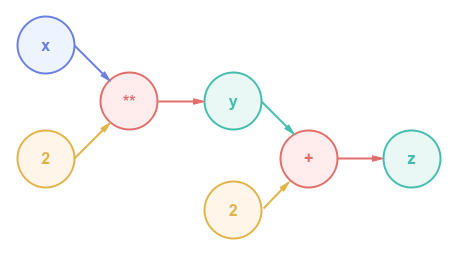
Let us look at a very simple example of computing the derivative $\Large{\frac{dz}{dx}}$ for the mathematical equation shown below:
$y = x^2$
$z = y + 2$
The following illustration depicts the computational graph for the above indicated mathematical equation:
To compute the derivative $\Large{\frac{dz}{dx}}$, one needs to use the chain rule as shown below:
$\Large{\frac{dz}{dx}}$ $= \Large{\frac{dz}{dy}}$ $. \Large{\frac{dy}{dx}}$
We know:
$\Large{\frac{dz}{dy}}$ $= \Large{\frac{d}{dy}}$ $(y + 2) = 1$
and:
$\Large{\frac{dy}{dx}}$ $= \Large{\frac{d}{dx}}$ $x^2 = 2.x$
Therefore:
$\Large{\frac{dz}{dx}}$ $= \Large{\frac{dz}{dy}}$ $. \Large{\frac{dy}{dx}}$ $= 2.x$
When $x = 2$:
$\Large{\frac{dz}{dx}}$ $= 2.x = 4$
To create the required tensors to represent the above mathematical equation, execute the following code snippet:
x = torch.tensor(2.0, requires_grad=True)
y = x ** 2
z = y + 2
The requires_grad option that is specified when creating the tensor $x$ in the code snippet above indicates that we desired the computation of the gradient for $x$.
To initiate the backward pass execution (backpropagation) and automatically compute and set the gradient for tensor $x$, execute the following code snippet:
z.backward()
To display the details about the tensor $x$, execute the following code snippet:
print(f'x value = {x.data}, x gradient = {x.grad}')
The following would be a typical output:
x value = 2.0, x gradient = 4.0
The tensor property data allows one to access the underlying data once the tensor is created, while the tensor property grad allows access to the computed gradient after the backward pass execution.
To access the gradient for the tensor $y$, execute the following code snippet:
print(f'TAKE-1 :: y value = {y.data}, y gradient = {y.grad}')
The following would be a typical output:
TAKE-1 :: y value = 4.0, y gradient = None
Hmm !!! Why is the gradient for the tensor $y$ ??? By default, tensors created without the requires_grad option is considered a non-leaf tensor and its gradient is not preserved during the backward pass execution. To change this behavior for debugging purpose, one can invoke the retain_grad() method on the non-leaf tensor.
To re-create the required tensors for the above mathematical equation and execute the backward pass, execute the following code snippet:
x = torch.tensor(2.0, requires_grad=True)
y = x ** 2
y.retain_grad()
z = y + 2
z.backward()
Now, to access the gradient for the tensor $y$, execute the following code snippet:
print(f'TAKE-2 :: y value = {y.data}, y gradient = {y.grad}')
The following would be a typical output:
TAKE-2 :: y value = 4.0, y gradient = 1.0
We will now move onto the final section on PyTorch model building basics.
PyTorch Model Basics
All the ingredients needed for building a neural network can be found in the PyTorch namespace torch.nn. To build a neural network model in PyTorch, one *MUST* create a model subclass, which inherits from the PyTorch base class nn.Module.
Let us consider a very simple linear equation $y = m.X + c$, where $X$ is the input feature, $m$ is the slope and $c$ is the intercept. This is basically a simple Linear Regression problem.
To import the necessary Python modules, execute the following code snippet:
from sklearn.model_selection import train_test_split
import matplotlib.pyplot as plt
import torch
from torch import nn
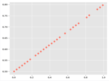
Let the slope $m = 0.3$ and let the intercept $c = 0.5$.
To create a sample dataset with the input $X$ and target $y$, execute the following code snippet:
X = torch.arange(0, 1, 0.03).unsqueeze(dim=1)
y = 0.3 * X + 0.5
To create the training and testing samples, execute the following code snippet:
X_train, X_test, y_train, y_test = train_test_split(X, y, test_size=0.2, random_state=101)
The following illustration shows the plot for the training set:
To create a Linear Regression for our simple use-case, execute the following code snippet:
num_features = 1
num_target = 1

class LinearRegressionModel(nn.Module):
  def __init__(self):
    super(LinearRegressionModel, self).__init__()
    self.linear_layer = nn.Linear(num_features, num_target)

  def forward(self, x: torch.Tensor) -> torch.Tensor:
    return self.linear_layer(x)
The layer nn.Linear performs a linear transformation $y = W^T.x + b$ on the incoming data. It takes in as input the number of input features and the number of targets. Based on the specified values, it automatically creates the associated weights and bias for the layer.
The method forward(self, x) defined in the base class nn.Module is *CRITICAL* and *MUST* be implemented - it defines the forward pass of the neural network.
To create an instance of the LinearRegressionModel and display its internal state, execute the following code snippet:
lr_model = LinearRegressionModel()
lr_model.state_dict()
The following would be a typical output:
OrderedDict([('linear_layer.weight', tensor([[-0.6039]])),
('linear_layer.bias', tensor([-0.0994]))])
To create an instance of the loss function, execute the following code snippet:
criterion = nn.L1Loss()
The class nn.L1Loss computes the mean absolute error $\vert predicted - actual \vert$.
To create an instance of the gradient descent function, execute the following code snippet:
optimizer = torch.optim.SGD(lr_model.parameters(), lr=0.01)
The class torch.optim.SGD(parameters, learning_rate) implements the necessary logic to adjust the parameters (weights and bias) adjustment using the gradient descent algorithm.
To implement the iterative training loop (epoch) in order to execute the forward pass to predict, compute the loss, and execute the backward pass to adjust the parameters, execute the following code snippet:
num_epochs = 351

for epoch in range(1, num_epochs):
  lr_model.train()
  optimizer.zero_grad()
  y_predict = lr_model(X_train)
  loss = criterion(y_predict, y_train)
  if epoch % 50 == 0:
    print(f'Epoch: {epoch}, Loss: {loss}')
  loss.backward()
  optimizer.step()
The following would be a typical output:
Epoch: 50, Loss: 0.4174691438674927
Epoch: 100, Loss: 0.12142442911863327
Epoch: 150, Loss: 0.0914655402302742
Epoch: 200, Loss: 0.06548042595386505
Epoch: 250, Loss: 0.039495326578617096
Epoch: 300, Loss: 0.013510189950466156
Epoch: 350, Loss: 0.004773879423737526
Notice the call to optimizer.zero_grad() - this is to zero the gradients computed from the earlier iteration.
Also, the to optimizer.step() is what performs the adjustments to the parameters using the gradient descent algorithm.
To display the values of the model parameters (the internal state of the model), execute the following code snippet:
lr_model.state_dict()
The following would be a typical output:
OrderedDict([('linear_layer.weight', tensor([[0.2925]])),
('linear_layer.bias', tensor([0.4961]))])
Notice how close the model parameters are to our original values of $m$ and $c$.
Before we wrap up, let us look at a simple Binary Classification problem. We will create and use synthetic data for this use-case. In addition, we will perform all the operations using the GPU.
To import the necessary Python module to create the synthetic data, execute the following code snippet:
from sklearn.datasets import make_blobs
from sklearn.metrics import accuracy_score
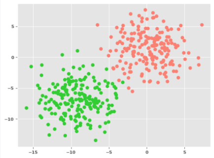
To create the synthetic data for the Binary Classification with two input features, execute the following code snippet:
num_samples = 500

np_Xc, np_yc = make_blobs(num_samples, n_features=2, centers=2, cluster_std=2.5, random_state=101)
To use the compute resource in a device agnostic way, execute the following code snippet:
device = 'cuda' if torch.cuda.is_available() else 'cpu'
If a CUDA based GPU is available, it will be leveraged. Else, it will default to the system CPU.
To create the tensor dataset on the GPU device, execute the following code snippet:
Xc = torch.tensor(np_Xc, dtype=torch.float, device=device)
yc = torch.tensor(np_yc, dtype=torch.float, device=device).unsqueeze(dim=1)
To create the training and testing samples, execute the following code snippet:
Xc_train, Xc_test, yc_train, yc_test = train_test_split(Xc, yc, test_size=0.2, random_state=101)
The following illustration shows the plot for the training set:
To create a Binary Classification for our simple use-case, execute the following code snippet:
num_features_2 = 2
num_target_2 = 1

class BinaryClassificationModel(nn.Module):
  def __init__(self):
    super(BinaryClassificationModel, self).__init__()
    self.hidden_layer = nn.Sequential(
      nn.Linear(num_features_2, num_target_2),
      nn.Sigmoid()
    )

  def forward(self, cx: torch.Tensor) -> torch.Tensor:
    return self.hidden_layer(cx)
The object nn.Sequential represents a container for layers in a neural network. The incoming data is forwarded thourgh each of the layers in this container. In this example, the incoming data is passed through a nn.Linear layer, followed by an activation layer nn.Sigmoid.
To create an instance of the BinaryClassificationModel on the GPU device and display its internal state, execute the following code snippet:
bc_model = BinaryClassificationModel()
bc_model.to(device)
bc_model.state_dict()
The following would be a typical output:
OrderedDict([('hidden_layer.0.weight',
  tensor([[-0.5786,  0.5476]], device='cuda:0')),
  ('hidden_layer.0.bias', tensor([-0.2978], device='cuda:0'))])
To create an instance of the loss function on the GPU device, execute the following code snippet:
criterion_2 = nn.BCELoss()
criterion_2.to(device)
The class nn.BCELoss computes the binary cross entropy error.
To create an instance of the gradient descent function, execute the following code snippet:
optimizer_2 = torch.optim.SGD(bc_model.parameters(), lr=0.05)
To implement the iterative training loop (epoch) in order to execute the forward pass to predict, compute the loss, and execute the backward pass to adjust the parameters, execute the following code snippet:
num_epochs_2 = 1001
for epoch in range(1, num_epochs_2):
  bc_model.train()
  optimizer_2.zero_grad()
  yc_predict = bc_model(Xc_train)
  loss = criterion_2(yc_predict, yc_train)
  if epoch % 50 == 0:
    print(f'Epoch: {epoch}, Loss: {loss}')
  loss.backward()
  optimizer_2.step()
The following would be a typical output:
Epoch: 100, Loss: 0.1626521497964859
Epoch: 150, Loss: 0.14181235432624817
Epoch: 200, Loss: 0.12650831043720245
Epoch: 250, Loss: 0.11473483592271805
Epoch: 300, Loss: 0.10540398955345154
Epoch: 350, Loss: 0.09782855957746506
Epoch: 400, Loss: 0.09155341982841492
Epoch: 450, Loss: 0.08626670390367508
Epoch: 500, Loss: 0.08174819499254227
Epoch: 550, Loss: 0.07783830165863037
Epoch: 600, Loss: 0.0744188204407692
Epoch: 650, Loss: 0.07140025496482849
Epoch: 700, Loss: 0.0687137320637703
Epoch: 750, Loss: 0.06630539149045944
Epoch: 800, Loss: 0.06413248926401138
Epoch: 850, Loss: 0.062160711735486984
Epoch: 900, Loss: 0.06036214530467987
Epoch: 950, Loss: 0.058713868260383606
Epoch: 1000, Loss: 0.05719691514968872
To display the values of the model parameters (the internal state of the model), execute the following code snippet:
bc_model.state_dict()
The following would be a typical output:
OrderedDict([('hidden_layer.0.weight',
  tensor([[-0.5084, -0.4961]], device='cuda:0')),
  ('hidden_layer.0.bias', tensor([-2.9599], device='cuda:0'))])
To predict the target values using the trained Binary Classification model, execute the following code snippet:
bc_model.eval()
with torch.no_grad():
  y_predict_2 = bc_model(Xc_test)
  y_predict_2 = torch.round(y_predict_2)
Note that in order to use the model for prediction, the model needs to be in an evaluation mode. This is achieved by invoking the method bc_model.eval() followed by the use of the context with torch.no_grad().
To display the model prediction accuracy, execute the following code snippet:
print(f'Accuracy: {accuracy_score(y_predict_2.cpu(), yc_test.cpu())}')
The following would be a typical output:
Accuracy: 0.99
Note that the PyTorch models demonstrated above were simple linear models.
References
Introduction to Deep Learning - Part 4
Introduction to Deep Learning - Part 3