Figure.1
| PolarSPARC |
Introduction to Deep Learning - Part 4
| Bhaskar S | 06/30/2023 |
Introduction
In Introduction to Deep Learning - Part 3 of this series, we got our hands dirty by building our own version of the perceptron and the neural network from scratch using Python.
In this article, we will continue our journey by introducing the very popular open source deep learning framework called PyTorch.
Installation and Setup
The installation and setup of PyTorch will be performed on a Ubuntu 22.04 LTS Linux desktop with a suitable NVidia graphics card and the Python programming language installed.
Open a Terminal window to perform the necessary installation step(s).
To install PyTorch, execute the following command:
$ sudo pip3 install torch torchaudio torchdata torchmetrics torchtext torchvision
This above command will install all the required dependencies along with the desired PyTorch packages.
Hands-on PyTorch
All the code snippets are executed in a Jupyter Notebook code cell.
PyTorch Basics
To import the PyTorch module, execute the following code snippet:
import torch
To check PyTorch was installed ok, execute the following code snippet:
torch.__version__
The following would be a typical output:
'2.0.0+cu117'
Notice the +cu117 in the output above. This implies that PyTorch is CUDA enabled.
To check if the GPU is accessible, execute the following code snippet:
torch.cuda.is_available()
The following would be a typical output:
True
The output above implies that PyTorch has access to the GPU device.
The core data structure in PyTorch is referred to as the Tensor and is an n-dimensional array structure. It can be thought of as similar to the ndarray structure in numpy. In other words, a Tensor can be used to represent a Scalar (zero dimension), or a Vector (one dimension), or a Matrix (two dimension), or a multi-dimensional structure (dimension greater than two).
The following are some of the features of Tensors:
Can operate using either the CPU or the GPU
Can be created using a Python list or a numpy ndarray
Attribute device indicates the device - CPU or GPU
Attribute dtype indicates the data type
Attribute shape indicates the dimensions
Support for all the basic mathematical operations (add, subtract, multiply, divide) on Tensors of same shape
Support for various mathematical functions (min, max, mean, sum, etc)
Support for various matrix related operations (multiply, transpose, svd, etc)
Support for various shape manipulation operations (reshape, squeeze, unsqueeze, etc)
Built-in support for automatically computing gradients (referred to as autograd)
To set the random seed for reproducibility, execute the following code snippet:
torch.manual_seed(101)
The following would be a typical output:
<torch._C.Generator at 0x7f17dddab7f0>
To create a scalar using a number, a vector and matrix using numpy ndarray, and a tensor using a Python list, execute the following code snippet:
scalar = torch.tensor(11)
vector = torch.tensor(np.array([13.0, 15.0]))
matrix = torch.tensor(np.array([
    [17.0, 19.0],
    [21.0, 23.0]
]), dtype=torch.float)
tensor = torch.tensor([[
    [25, 27, 29],
    [31, 33, 35],
    [37, 39, 41]
],
[
    [43, 49, 55],
    [45, 51, 57],
    [47, 53, 59]
]], dtype=torch.float, device='cuda')
Notice how one can specify the data type and the device from the above code snippet. The value of cuda implies the NVidia GPU device.
To display the details about the scalar, execute the following code snippet:
print(f'Scalar: {scalar}, Shape: {scalar.shape}, Type: {scalar.dtype}, Device: {scalar.device}')
The following would be a typical output:
Scalar: 11, Shape: torch.Size([]), Type: torch.int64, Device: cpu
To display the details about the vector, execute the following code snippet:
print(f'Vector: {vector}, Shape: {vector.shape}, Type: {vector.dtype}, Device: {vector.device}')
The following would be a typical output:
Vector: tensor([13., 15.], dtype=torch.float64), Shape: torch.Size([2]), Type: torch.float64, Device: cpu
To display the details about the matrix, execute the following code snippet:
print(f'Matrix: {matrix}, Shape: {matrix.shape}, Type: {matrix.dtype}, Device: {matrix.device}')
The following would be a typical output:
Matrix: tensor([[17., 19.],
  [21., 23.]]), Shape: torch.Size([2, 2]), Type: torch.float32, Device: cpu
To display the details about the tensor, execute the following code snippet:
print(f'Tensor: {tensor}, Shape: {tensor.shape}, Type: {tensor.dtype}, Device: {tensor.device}')
The following would be a typical output:
Tensor: tensor([[[25., 27., 29.],
  [31., 33., 35.],
  [37., 39., 41.]],

  [[43., 49., 55.],
  [45., 51., 57.],
  [47., 53., 59.]]], device='cuda:0'), Shape: torch.Size([2, 3, 3]), Type: torch.float32, Device: cuda:0
The default float data type in PyTorch is *float32*, while in numpy it is *float64*
To access the individual elements of a Tensor, execute the following code snippet:
print(f'vector[1] = {vector[1]}, matrix[1][0] = {matrix[1][0]}, matrix[1, 0] = {matrix[1, 0]},'
  f'tensor[0][1][2] = {tensor[0][1][2]}, tensor[0, 1, 2] = {tensor[0, 1, 2]}')
The following would be a typical output:
vector[1] = 15.0, matrix[1][0] = 21.0, matrix[1, 0] = 21.0,tensor[0][1][2] = 35.0, tensor[0, 1, 2] = 35.0
To access the sub-Tensors within a Tensor, execute the following code snippet:
print(f'matrix[0] = {matrix[0]}, matrix[:, 1] = {matrix[:, 1]}, tensor[0] = {tensor[0]}, tensor[0][1] = {tensor[0][1]}, '
  f'tensor[:, :, 1] = {tensor[:, :, 1]}')
The following would be a typical output:
matrix[0] = tensor([17., 19.]), matrix[:, 1] = tensor([19., 23.]), tensor[0] = tensor([[25., 27., 29.],
  [31., 33., 35.],
  [37., 39., 41.]], device='cuda:0'), tensor[0][1] = tensor([31., 33., 35.], device='cuda:0'), tensor[:, :, 1] = tensor([[27., 33., 39.],
  [49., 51., 53.]], device='cuda:0')
To create a vector Tensor of a specific type within a range in steps, execute the following code snippet:
vector1 = torch.arange(1, 101, step=11, dtype=torch.float32)
vector1
The following would be a typical output:
tensor([ 1., 12., 23., 34., 45., 56., 67., 78., 89., 100.])
To create a Tensor of shape 3x3 with random values, execute the following code snippet:
tensor1 = torch.rand(size=(3, 3))
tensor1
The following would be a typical output:
tensor([[0.1980, 0.4503, 0.0909],
  [0.8872, 0.2894, 0.0186],
  [0.9095, 0.3406, 0.4309]])
To create a Tensor of shape 3x3x3 with zero values, execute the following code snippet:
zeros_tensor = torch.zeros(size=(3, 3, 3))
zeros_tensor
The following would be a typical output:
tensor([[[0., 0., 0.],
   [0., 0., 0.],
   [0., 0., 0.]],

  [[0., 0., 0.],
   [0., 0., 0.],
   [0., 0., 0.]],

  [[0., 0., 0.],
   [0., 0., 0.],
   [0., 0., 0.]]])
To create a Tensor of shape 3x3x3 with all one values, execute the following code snippet:
ones_tensor = torch.ones(size=(3, 3, 3))
ones_tensor
The following would be a typical output:
tensor([[[1., 1., 1.],
   [1., 1., 1.],
   [1., 1., 1.]],

  [[1., 1., 1.],
   [1., 1., 1.],
   [1., 1., 1.]],

  [[1., 1., 1.],
   [1., 1., 1.],
   [1., 1., 1.]]])
We will now move onto the next section on Tensors related to mathematical operations.
Tensor Mathematical Operations
To create a vector of shape 1x3 and a matrix of shape 3x3, execute the following code snippet:
vector2 = torch.rand(size=(1, 3))
matrix1 = torch.rand(size=(3, 3))
print(f'vector2 = {vector2}, matrix1 = {matrix1}')
The following would be a typical output:
vector2 = tensor([[0.6389, 0.3944, 0.2462]]), matrix1 = tensor([[0.7276, 0.8310, 0.6744],
   [0.0299, 0.6592, 0.3304],
   [0.6563, 0.5190, 0.0596]])
To multiply the vector by the matrix, execute the following code snippet:
vector2 * matrix1
The following would be a typical output:
tensor([[0.4649, 0.3277, 0.1661],
   [0.0191, 0.2600, 0.0814],
   [0.4193, 0.2047, 0.0147]])
To multiply two matrices of shapes 2x3 and 3x2 (note the inner dimensions must match), execute the following code snippet:
matrix2 = torch.ones(size=(2, 3))
matrix2 *= 5
matrix3 = torch.ones(size=(3, 2))
matrix2 *= 2
matrix2 @ matrix3
The following would be a typical output:
tensor([[30., 30.],
   [30., 30.]])
The @ operator is for matrix multiplication. One could also use the following two methods to perform the same operation.
torch.matmul(matrix2, matrix3)
torch.mm(matrix2, matrix3)
To perform the transpose operation on the matrix of shape 3x2, execute the following code snippet:
matrix3.T
The following would be a typical output:
tensor([[2., 2., 2.],
   [2., 2., 2.]])
For the next set of operations, let us consider the following Tensor of shape 3x2x3:
tensor2 = torch.tensor([
  [
    [10, 11, 12],
    [13, 14, 15]
  ],
  [
    [20, 21, 22],
    [23, 24, 25]
  ],
  [
    [30, 31, 32],
    [33, 34, 35]
  ]
], dtype=torch.float)
Dimension 0 is each of the 3 sub-tensors (matrices), dimension 1 are the rows, and dimension 2 are the columns.
To perform a data type conversion of tensor2 elements to int32 type, execute the following code snippet:
tensor2.to(dtype=torch.int32)
The following would be a typical output:
tensor([[[10, 11, 12],
   [13, 14, 15]],

  [[20, 21, 22],
   [23, 24, 25]],

  [[30, 31, 32],
   [33, 34, 35]]], dtype=torch.int32)
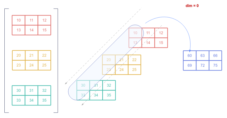
To perform the a sum operation on tensor2 along dimension 0, execute the following code snippet:
tensor2.sum(dim=0)
The following would be a typical output:
tensor([[60., 63., 66.],
  [69., 72., 75.]])
The following illustration depicts the sum operation visually:
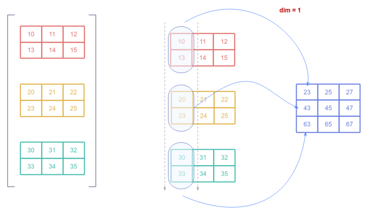
To perform the a sum operation on tensor2 along dimension 1, execute the following code snippet:
tensor2.sum(dim=1)
The following would be a typical output:
tensor([[23., 25., 27.],
  [43., 45., 47.],
  [63., 65., 67.]])
The following illustration depicts the sum operation visually:
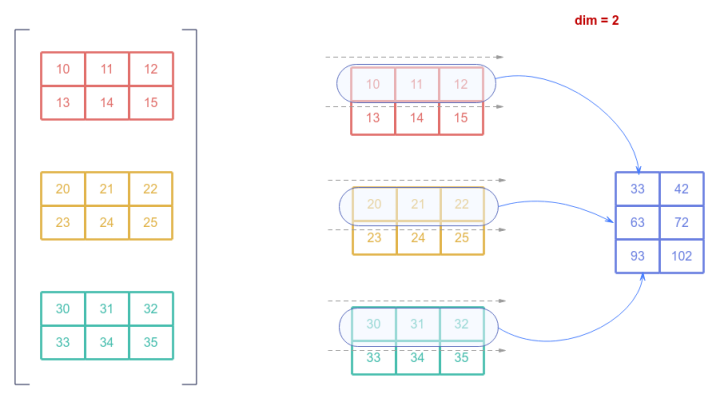
To perform the a sum operation on tensor2 along dimension 2, execute the following code snippet:
tensor2.sum(dim=2)
The following would be a typical output:
tensor([[ 33.,  42.],
  [ 63.,  72.],
  [ 93., 102.]])
The following illustration depicts the sum operation visually:
To perform the a mean operation on tensor2 along dimension 1, execute the following code snippet:
tensor2.mean(dim=1)
The following would be a typical output:
tensor([[11.5000, 12.5000, 13.5000],
  [21.5000, 22.5000, 23.5000],
  [31.5000, 32.5000, 33.5000]])
There are more than 300+ mathematical functions defined in PyTorch.
References