Figure.1
| PolarSPARC |
Introduction to Deep Learning - Part 3
| Bhaskar S | 06/18/2023 |
Introduction
In Introduction to Deep Learning - Part 2 of this series, we introduced the concepts on feed forward network, loss function, gradient descent, and backpropagation .
In this article, we will continue our journey, by implementing our own version of a perceptron and a neural network from scratch using Python, to better understand the core concepts.
Perceptron From Scratch
From Introduction to Deep Learning - Part 1 of this series, we learnt that a perceptron simply behaves like a linear classifier.
Also, the default activation function $\sigma$ associated with a perceptron is a binary step function, which outputs two discrete values - a $0$ if $\sigma(x) \le 0$ and a $1$ if $\sigma(x) \gt 0$.
The following code snippet shows the implementation of the step activation function:
import numpy as np

def activation_step(x):
  return np.where(x > 0.0, 1, 0)
From Introduction to Deep Learning - Part 2 of this series, we learnt how to minimize the loss (or cost) using gradient descent. The idea is to compute the loss for each iteration of the training and progressively adjust the bias and the weights of the perceptron till the loss is minimized.
The following code snippet shows the implementation of the perceptron:
import numpy as np

class MyPerceptron:
#
# Params:
#     eta        - learning rate
#     epochs     - number of iterations
#     activation - activation function
#
def __init__(self, eta=0.01, epochs=500, activation=activation_step):
    self.eta = eta
    self.epochs = epochs
    self.activation_func = activation
    self.weights = None
    self.bias = np.random.random(1)

def fit(self, X_f, y_f):
    n_samples, n_features = X_f.shape

    # Run target values through the activation function
    ay = self.activation_func(y_f)

    # Initialize the weights for all the features
    self.weights = np.random.random(n_features)

    for epoch in range(self.epochs):
        for i in range(n_samples):
            # Predict the outcomes
            yp = np.dot(X_f[i], self.weights) + self.bias

            # Run predicted values through the activation function
            ayp = self.activation_func(yp)

            # Compute the loss = (predicted - actual)
            loss = ayp - ay[i]
            if loss != 0:
                # Adjust the weights and bias
                adjustment = self.eta * loss
                self.weights -= adjustment * X_f[i]
                self.bias -= adjustment

def predict(self, X_p):
    # Predict the outcomes
    yp = np.dot(X_p, self.weights) + self.bias

    # Return the predicted values after running through the activation function
    return self.activation_func(yp)

def info(self):
    print('Bias:', self.bias, ', Weights:', self.weights)
Now, to test our implementation of the perceptron, we will create about $100$ data samples that belongs to one of the two classes (binary classification).
The following code snippet shows how to generate the data set and split it into a training and a testing set:
from sklearn import datasets
from sklearn.model_selection import train_test_split

X, y = datasets.make_blobs(n_samples=100, n_features=2, centers=[[-3.5, -2.0], [2.5, 3.5]], cluster_std=2.25, random_state=5)
X_train, X_test, y_train, y_test = train_test_split(X, y, test_size=0.25, random_state=5)
The following code snippet shows how to instantiate our perceptron class and display its internal state:
my_per = MyPerceptron()
my_per.info()
Executing the above code snippet would result in the following typical output:
Bias: [0.07630829] , Weights: None
The following code snippet shows how to train our perceptron using the training data set and then display its internal state:
my_per.fit(X_train, y_train)
my_per.info()
Executing the above code snippet would result in the following typical output:
Bias: [0.02630829] , Weights: [0.8253873 0.32945949]
Notice from Output.2 above the adjusted bias and weights post training.
The following code snippet shows how to predict outcomes using our perceptron with the testing data set and display prediction accuracy:
y_predict = my_per.predict(X_test)

print('Accuracy:', np.sum(y_predict == y_test)/len(y_test))
Executing the above code snippet would result in the following typical output:
Accuracy: 0.84
Notice from Output.3 above that the prediction rate is about 84 %, which is not bad at all !!!
Neural Network From Scratch
Our implementation of the neural network will be used to solve a binary classification problem. This implies we can leverage the sigmoid function as the activation function . From Introduction to Deep Learning - Part 1 of this series, we know that the sigmoid function is a non-linear activation function, that produces an output in the range of $0$ to $1$ for a given input.
In mathematical terms:
$y = \sigma(x) = \Large{\frac{1}{1 + e^{-x}}}$ $..... \color{red}\textbf{(1)}$
The sigmoid activation function has a very interesting behavior with respect to finding its derivative.
In mathematical sense:
$\Large{\frac{d\sigma}{dx}}$ $= \Large{\frac{d}{dx}}$ $\Large{(\frac{1}{1 + e^{-x}})}$ $= \Large{ \frac{d}{dx}}$ $(1 + e^{-x})^{-1}$ $..... \color{red}\textbf{(2)}$
Given that equation $\color{red}\textbf{(2)}$ is a composite function, it involves the chain rule. That is:
$\Large{\frac{d}{dx}}$ $(1 + e^{-x})^{-1}$ $= (-1).(1 + e^{-x})^{-2}.$ $\Large{\frac{d}{dx}}$ $(1 + e^{-x})$
That is:
$\Large{\frac{d}{dx}}$ $(1 + e^{-x})^{-1}$ $= (-1).(1 + e^{-x})^{-2}.$ $\Large{\frac{d}{dx}}$ $(e^{-x})$ $= (-1).(1 + e^{-x})^{-2}.e^{-x}.$ $\Large{\frac{d}{dx}}$ $(-x)$
Or:
$\Large{\frac{d}{dx}}$ $(1 + e^{-x})^{-1}$ $= (-1).(1 + e^{-x})^{-2}.e^{-x}.(-1)$ $= e^{-x}.(1 + e^{-x})^{-2}$
In other words:
$\Large{\frac{d}{dx}}$ $(1 + e^{-x})^{-1}$ $= \Large{\frac{e^{-x}}{(1 + e^{-x})^2}}$ $= \Large{ \frac{e^{-x} + 1 - 1}{(1 + e^{-x})^2}}$ $= \Large{\frac{1}{(1 + e^{-x})^{-1}}.\frac{1 + e^{-x} - 1}{(1 + e^{-x})^{-1}}}$
Rewriting:
$\Large{\frac{d}{dx}}$ $(1 + e^{-x})^{-1}$ $= \Large{\frac{1}{(1 + e^{-x})^{-1}}. (\frac{(1 + e^{-x})^{-1}}{(1 + e^{-x})^{-1}} - \frac{1}{(1 + e^{-x})^{-1}})}$ $= \Large{\frac{1}{(1 + e^{-x})^{-1}}}$ $. (1 - \Large{\frac{1}{(1 + e^{-x})^{-1}}} \normalsize{)}$
Simplifing, we get:
$\Large{\frac{d}{dx}}$ $(1 + e^{-x})^{-1}$ $= \sigma(x).(1 - \sigma(x))$ $..... \color{red} \textbf{(3)}$
From the equation $\color{red}\textbf{(3)}$ above, we can infer the derivative of the sigmoid function can be computed using the sigmoid function itself.
The following code snippet shows the implementation of the sigmoid activation function:
def activation_sigmoid(z):
  return 1 / (1 + math.exp(-z))
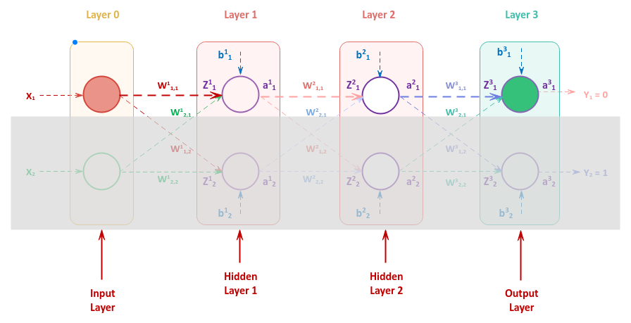
In order to understand the quantity by which to adjust the bias and the weight s of the various neurons in a neural network, let us once again refer to the following illustration of the neural network with an input layer with two inputs, two hidden layers each consisting of two neurons, and an output layer with two outputs
We will focus on the upper neurons and ignore the shaded area to flush the details.
To adjust the weight $W_{1,1}^3$, we need to compute the gradient for $\Large{\frac{\partial{L}}{\partial{W_{1,1}^3}}}$.
Once we have the gradient for $\Large{\frac{\partial{L}}{\partial{W_{1,1}^3}}}$, we can adjust the weight $W_{1,1}^3$ as follows:
$W_{1,1}^3 = W_{1,1}^3 -$ $\eta * \Large{\frac{\partial{L}}{\partial{W_{1,1}^3}}}$ $..... \color{red} \textbf{(4)}$
We can compute the gradient for $\Large{\frac{\partial{L}}{\partial{W_{1,1}^3}}}$ as follows:
$\Large{\frac{\partial{L}}{\partial{W_{1,1}^3}}}$ $= \Large{\frac{\partial{Z_1^3}}{\partial{W_{1,1}^3}}}$ $. \Large{\frac{\partial{a_1^3}}{\partial{Z_1^3}}}$ $. \Large{\frac{\partial{L}}{\partial{a_1^3}}}$ $..... \color{red} \textbf{(5)}$
The loss (or the cost) $L$ for one iteration of training is the average of the sum of mean squared errors.
That is:
$L = \Large{\frac{1}{n}}$ $. \sum_{i=1}^n (predicted - actual)^2$ $= \Large{\frac{1}{n}}$ $. \sum_{i=1}^n (a_1^3 - Y_1)^2$ $..... \color{red}\textbf{(6)}$
where $n$ is the number of samples in the training data set.
From equation $\color{red}\textbf{(6)}$, we can compute $\Large{\frac{\partial{L}}{\partial{a_1^3}}}$ as follows:
$\Large{\frac{\partial{L}}{\partial{a_1^3}}}$ $= \Large{\frac{2}{n}}$ $. \sum_{i=1}^n (a_1^3 - Y_1)$ $..... \color{red}\textbf{(7)}$
where $n$ is the number of samples in the training data set.
Some implementations of the loss function L divide the sum of mean squared errors by 2 instead of n, so that the factor 2 cancels out when the derivative is computed. For our implementation, we will use this approach as well
The activation (the sigmoid function) $a$ is computed using the weighted sum of inputs $z$ as follows:
$a = \sigma(z) = \Large{\frac{1}{(1 + e^{-z})}}$
where $z$ is the weighted sum of inputs from the neuron.
From equation $\color{red}\textbf{(3)}$ above, we can compute $\Large{\frac{\partial{a_1^3}}{\partial{Z_1^3}}}$ as follows:
$\Large{\frac{\partial{a_1^3}}{\partial{Z_1^3}}}$ $= \sigma(Z_1^3).(1 - \sigma(Z_1^3))$ $..... \color {red}\textbf{(8)}$
The weighted sum $z$ for a neuron with bias $b$ and inputs $x_j$ with corresponding weights $W_j$ is computed as follows:
$z = b + \sum_{j=1}^m x_j.W_j$ $..... \color{red}\textbf{(9)}$
where $m$ is the number of inputs into the neuron.
Using equation $\color{red}\textbf{(9)}$, we can compute $Z_1^3$ as follows:
$Z_1^3 = b_1^3 + W_{1,1}^3.a_1^2 + W_{2,1}^3.a_2^2$ $..... \color{red}\textbf{(10)}$
From equation $\color{red}\textbf{(10)}$, we can compute $\Large{\frac{\partial{Z_1^3}}{\partial{W_{1,1}^3}}}$ as follows:
$\Large{\frac{\partial{Z_1^3}}{\partial{W_{1,1}^3}}}$ $= a_1^2$ $..... \color{red}\textbf{(11)}$
Substituting the equations $\color{red}\textbf{(11)}$, $\color{red}\textbf{(8)}$, and $\color{red}\textbf{(7)}$ into the equation $\color{red}\textbf{(5)}$, we can now compute $\Large{\frac{\partial{L}}{\partial{W_{1,1}^3}}}$ as follows:
$\Large{\frac{\partial{L}}{\partial{W_{1,1}^3}}}$ $= a_1^2.\sigma(Z_1^3).(1 - \sigma(Z_1^3))$ $. \Large{\frac{2}{n}}$ $. \sum_{i=1}^n (a_1^3 - Y_1)$ $..... \color{red}\textbf{(12)}$
To adjust the bias $b_1^3$, we need to compute the gradient for $\Large{\frac{\partial{L}}{\partial{b_1^3}}}$.
Once we have the gradient for $\Large{\frac{\partial{L}}{\partial{b_1^3}}}$, we can adjust the bias $b_1^3$ as follows:
$b_1^3 = b_1^3 -$ $\eta * \Large{\frac{\partial{L}}{\partial{b_1^3}}}$ $..... \color{red}\textbf{(13)}$
We can compute the gradient for $\Large{\frac{\partial{L}}{\partial{b_1^3}}}$ as follows:
$\Large{\frac{\partial{L}}{\partial{b_1^3}}}$ $= \Large{\frac{\partial{Z_1^3}}{\partial{b_1^3}}}$ $. \Large{\frac{\partial{a_1^3}}{\partial{Z_1^3}}}$ $. \Large{\frac{\partial{L}}{\partial{a_1^3}}}$ $..... \color{red} \textbf{(14)}$
From equation $\color{red}\textbf{(10)}$ above, we can compute $\Large{\frac{\partial{Z_1^3}}{\partial{b_1^3}}}$ as follows:
$\Large{\frac{\partial{Z_1^3}}{\partial{b_1^3}}}$ $= 1$ $..... \color{red}\textbf{(15)}$
Substituting the equations $\color{red}\textbf{(15)}$, $\color{red}\textbf{(8)}$, and $\color{red}\textbf{(7)}$ into the equation $\color{red}\textbf{(14)}$, we can now compute $\Large{\frac{\partial{L}}{\partial{b_1^3}}}$ as follows:
$\Large{\frac{\partial{L}}{\partial{b_1^3}}}$ $= \sigma(Z_1^3).(1 - \sigma(Z_1^3))$ $. \Large{\frac{2}{n}}$ $. \sum_{i=1}^n (a_1^3 - Y_1)$ $..... \color{red}\textbf{(16)}$
From the equations $\color{red}\textbf{(12)}$ and $\color{red}\textbf{(16)}$ above, we see some common terms, which simply represent the gradient of the output layer for the first input. We can represent the common terms using $\delta_1^3$ as follows:
$\delta_1^3 = \Large{\frac{\partial{a_1^3}}{\partial{Z_1^3}}}$ $. \Large{\frac{\partial{L}}{\partial {a_1^3}}}$ $= \sigma(Z_1^3).(1 - \sigma(Z_1^3))$ $. \Large{\frac{2}{n}}$ $. \sum_{i=1}^n (a_1^3 - Y_1)$ $..... \color{red} \textbf{(17)}$
Substituting $\color{red}\textbf{(17)}$ into equations $\color{red}\textbf{(12)}$ and $\color{red}\textbf{(16)}$, we get:
$\Large{\frac{\partial{L}}{\partial{W_{1,1}^3}}}$ $= \bbox[pink,2pt]{a_1^2.\delta_1^3}$ $..... \color {red}\textbf{(18)}$
and
$\Large{\frac{\partial{L}}{\partial{b_1^3}}}$ $= \bbox[pink,2pt]{\delta_1^3}$ $..... \color{red} \textbf{(19)}$
Moving on, in order to adjust the weight $W_{1,1}^2$, we need to compute the gradient for $\Large{\frac{\partial{L}}{\partial {W_{1,1}^2}}}$.
Once we have the gradient for $\Large{\frac{\partial{L}}{\partial{W_{1,1}^2}}}$, we can adjust the weight $W_{1,1}^2$ as follows:
$W_{1,1}^2 = W_{1,1}^2 -$ $\eta * \Large{\frac{\partial{L}}{\partial{W_{1,1}^2}}}$ $..... \color{red} \textbf{(20)}$
We can compute the gradient for $\Large{\frac{\partial{L}}{\partial{W_{1,1}^2}}}$ as follows:
$\Large{\frac{\partial{L}}{\partial{W_{1,1}^2}}}$ $= \Large{\frac{\partial{Z_1^2}}{\partial{W_{1,1}^2}}}$ $. \Large{\frac{\partial{a_1^2}}{\partial{Z_1^2}}}$ $. \Large{\frac{\partial{Z_1^3}}{\partial{a_1^2}}}$ $. \Large{\frac{\partial {a_1^3}}{\partial{Z_1^3}}}$ $. \Large{\frac{\partial{L}}{\partial{a_1^2}}}$ $..... \color{red}\textbf{(21)}$
Substituting $\color{red}\textbf{(17)}$ into equation $\color{red}\textbf{(21)}$, we get:
$\Large{\frac{\partial{L}}{\partial{W_{1,1}^2}}}$ $= \Large{\frac{\partial{Z_1^2}}{\partial{W_{1,1}^2}}}$ $. \Large{\frac{\partial{a_1^2}}{\partial{Z_1^2}}}$ $. \Large{\frac{\partial{Z_1^3}}{\partial{a_1^2}}}$ $. \delta_1^3$ $..... \color{red}\textbf{(22)}$
From equation $\color{red}\textbf{(10)}$ above, we can compute $\Large{\frac{\partial{Z_1^3}}{\partial{a_1^2}}}$ as follows:
$\Large{\frac{\partial{Z_1^3}}{\partial{a_1^2}}}$ $= W_{1,1}^3$ $..... \color{red}\textbf{(23)}$
From equation $\color{red}\textbf{(3)}$ above, we can compute $\Large{\frac{\partial{a_1^2}}{\partial{Z_1^2}}}$ as follows:
$\Large{\frac{\partial{a_1^2}}{\partial{Z_1^2}}}$ $= \sigma(Z_1^2).(1 - \sigma(Z_1^2))$ $..... \color {red}\textbf{(24)}$
Using equation $\color{red}\textbf{(9)}$, we can compute $Z_1^2$ as follows:
$Z_1^2 = b_1^2 + W_{1,1}^2.a_1^1 + W_{2,1}^2.a_2^1$ $..... \color{red}\textbf{(25)}$
From equation $\color{red}\textbf{(25)}$, we can compute $\Large{\frac{\partial{Z_1^2}}{\partial{W_{1,1}^2}}}$ as follows:
$\Large{\frac{\partial{Z_1^2}}{\partial{W_{1,1}^2}}}$ $= a_1^1$ $..... \color{red}\textbf{(26)}$
Substituting the equations $\color{red}\textbf{(26)}$, $\color{red}\textbf{(24)}$, and $\color{red}\textbf{(23)}$ into the equation $\color{red}\textbf{(22)}$, we can now compute $\Large{\frac{\partial{L}}{\partial{W_{1,1}^2}}}$ as follows:
$\Large{\frac{\partial{L}}{\partial{W_{1,1}^2}}}$ $= \bbox[pink,2pt]{a_1^1.\sigma(Z_1^2).(1 - \sigma(Z_1^2)).W_{1,1}^3.\delta_1^3}$ $..... \color{red}\textbf{(27)}$
Next, to adjust the bias $b_1^2$, we need to compute the gradient for $\Large{\frac{\partial{L}}{\partial{b_1^2}}}$.
Once we have the gradient for $\Large{\frac{\partial{L}}{\partial{b_1^2}}}$, we can adjust the bias $b_1^2$ as follows:
$b_1^2 = b_1^2 -$ $\eta * \Large{\frac{\partial{L}}{\partial{b_1^2}}}$ $..... \color{red}\textbf{(28)}$
We can compute the gradient for $\Large{\frac{\partial{L}}{\partial{b_1^2}}}$ as follows:
$\Large{\frac{\partial{L}}{\partial{b_1^2}}}$ $= \Large{\frac{\partial{Z_1^2}}{\partial{b_1^2}}}$ $. \Large{\frac{\partial{a_1^2}}{\partial{Z_1^2}}}$ $. \Large{\frac{\partial{Z_1^3}}{\partial{a_1^2}}}$ $. \Large{\frac{\partial {a_1^3}}{\partial{Z_1^3}}}$ $. \Large{\frac{\partial{L}}{\partial{a_1^3}}}$ $..... \color{red}\textbf{(29)}$
Substituting $\color{red}\textbf{(17)}$ into equation $\color{red}\textbf{(29)}$, we get:
$\Large{\frac{\partial{L}}{\partial{b_1^2}}}$ $= \Large{\frac{\partial{Z_1^2}}{\partial{b_1^2}}}$ $. \Large{\frac{\partial{a_1^2}}{\partial{Z_1^2}}}$ $. \Large{\frac{\partial{Z_1^3}}{\partial{a_1^2}}}$ $. \delta_1^3$ $..... \color{red}\textbf{(30)}$
From equation $\color{red}\textbf{(25)}$ above, we can compute $\Large{\frac{\partial{Z_1^2}}{\partial{b_1^2}}}$ as follows:
$\Large{\frac{\partial{Z_1^2}}{\partial{b_1^2}}}$ $= 1$ $..... \color{red}\textbf{(31)}$
Substituting the equations $\color{red}\textbf{(31)}$, $\color{red}\textbf{(24)}$, and $\color{red}\textbf{(23)}$ into the equation $\color{red}\textbf{(30)}$, we can now compute $\Large{\frac{\partial{L}}{\partial{b_1^2}}}$ as follows:
$\Large{\frac{\partial{L}}{\partial{b_1^2}}}$ $= \bbox[pink,2pt]{\sigma(Z_1^2).(1 - \sigma(Z_1^2)) .W_{1,1}^3.\delta_1^3}$ $..... \color{red}\textbf{(32)}$
From the equations $\color{red}\textbf{(27)}$ and $\color{red}\textbf{(32)}$ above, we again see some common terms, which represents the gradient from the second hidden layer for the first input. We can represent the common terms using $\delta_1^2$ as follows:
$\delta_1^2 = \Large{\frac{\partial{a_1^2}}{\partial{Z_1^2}}}$ $. \Large{\frac{\partial{Z_1^3}} {\partial{a_1^2}}}$ $= \sigma(Z_1^2).(1 - \sigma(Z_1^2)).W_{1,1}^3$ $..... \color{red}\textbf{(33)}$
Substituting $\color{red}\textbf{(33)}$ into equations $\color{red}\textbf{(27)}$ and $\color{red}\textbf{(32)}$, we get:
$\Large{\frac{\partial{L}}{\partial{W_{1,1}^2}}}$ $= \bbox[pink,2pt]{a_1^1.\delta_1^2.\delta_1^3}$ $..... \color{red}\textbf{(34)}$
and
$\Large{\frac{\partial{L}}{\partial{b_1^2}}}$ $= \bbox[pink,2pt]{\delta_1^2.\delta_1^3}$ $..... \color{red}\textbf{(35)}$
One last time, in order to adjust the weight $W_{1,1}^1$, we need to compute the gradient for $\Large{\frac{\partial{L}} {\partial{W_{1,1}^1}}}$.
Once we have the gradient for $\Large{\frac{\partial{L}}{\partial{W_{1,1}^1}}}$, we can adjust the weight $W_{1,1}^1$ as follows:
$W_{1,1}^1 = W_{1,1}^1 -$ $\eta * \Large{\frac{\partial{L}}{\partial{W_{1,1}^1}}}$ $..... \color {red}\textbf{(36)}$
We can compute the gradient for $\Large{\frac{\partial{L}}{\partial{W_{1,1}^1}}}$ as follows:
$\Large{\frac{\partial{L}}{\partial{W_{1,1}^1}}}$ $= \Large{\frac{\partial{Z_1^1}}{\partial{W_{1,1} ^1}}}$ $.\Large{\frac{\partial{a_1^1}}{\partial{Z_1^1}}}$ $.\Large{\frac{\partial{Z_1^2}}{\partial{a_1^1}}}$ $.\Large{\frac {\partial{a_1^2}}{\partial{Z_1^2}}}$ $.\Large{\frac{\partial{Z_1^3}}{\partial{a_1^2}}}$ $.\Large{\frac{\partial{a_1^3}} {\partial{Z_1^3}}}$ $.\Large{\frac{\partial{L}}{\partial{a_1^2}}}$ $..... \color{red}\textbf{(37)}$
Substituting $\color{red}\textbf{(17)}$ and $\color{red}\textbf{(33)}$ into equation $\color{red}\textbf{(37)}$, we get:
$\Large{\frac{\partial{L}}{\partial{W_{1,1}^1}}}$ $= \Large{\frac{\partial{Z_1^1}}{\partial{W_{1,1} ^1}}}$ $.\Large{\frac{\partial{a_1^1}}{\partial{Z_1^1}}}$ $.\Large{\frac{\partial{Z_1^2}}{\partial{a_1^1}}}$ $.\delta_1^2. \delta_1^3$ $..... \color{red}\textbf{(38)}$
We are not going to compute all the partial derivative terms as they follow the patterns discussed earlier. The end result for computing $\Large{\frac{\partial{L}}{\partial{W_{1,1}^1}}}$ is as follows:
$\Large{\frac{\partial{L}}{\partial{W_{1,1}^1}}}$ $= \bbox[pink,2pt]{x_1.\sigma(Z_1^1).(1 - \sigma (Z_1^1)).W_{1,1}^2.\delta_1^2.\delta_1^3}$ $..... \color{red}\textbf{(39)}$
One last time, in order to adjust the bias $b_1^1$, we need to compute the gradient for $\Large{\frac{\partial{L}}{\partial {b_1^1}}}$.
Once we have the gradient for $\Large{\frac{\partial{L}}{\partial{b_1^1}}}$, we can adjust the bias $b_1^1$ as follows:
$b_1^1 = b_1^1 -$ $\eta * \Large{\frac{\partial{L}}{\partial{b_1^1}}}$ $..... \color{red}\textbf {(40)}$
We can compute the gradient for $\Large{\frac{\partial{L}}{\partial{b_1^1}}}$ as follows:
$\Large{\frac{\partial{L}}{\partial{b_1^1}}}$ $= \Large{\frac{\partial{Z_1^1}}{\partial{b_1^1}}}$ $.\Large{\frac{\partial{a_1^1}}{\partial{Z_1^1}}}$ $.\Large{\frac{\partial{Z_1^2}}{\partial{a_1^1}}}$ $.\Large{\frac {\partial{a_1^2}}{\partial{Z_1^2}}}$ $.\Large{\frac{\partial{Z_1^3}}{\partial{a_1^2}}}$ $.\Large{\frac{\partial{a_1^3}} {\partial{Z_1^3}}}$ $.\Large{\frac{\partial{L}}{\partial{a_1^2}}}$ $..... \color{red}\textbf{(41)}$
Substituting $\color{red}\textbf{(17)}$ and $\color{red}\textbf{(33)}$ into equation $\color{red}\textbf{(41)}$, we get:
$\Large{\frac{\partial{L}}{\partial{b_1^1}}}$ $= \Large{\frac{\partial{Z_1^1}}{\partial{b_1^1}}}$ $.\Large{\frac{\partial{a_1^1}}{\partial{Z_1^1}}}$ $.\Large{\frac{\partial{Z_1^2}}{\partial{a_1^1}}}$ $.\delta_1^2.\delta_1^3$ $..... \color{red}\textbf{(42)}$
We are not going to compute all the partial derivative terms as they follow the patterns discussed earlier. The end result for computing $\Large{\frac{\partial{L}}{\partial{b_1^1}}}$ is as follows:
$\Large{\frac{\partial{L}}{\partial{b_1^1}}}$ $= \bbox[pink,2pt]{\sigma(Z_1^1).(1 - \sigma(Z_1^1)) .W_{1,1}^2.\delta_1^2.\delta_1^3}$ $..... \color{red}\textbf{(43)}$
From the equations $\color{red}\textbf{(39)}$ and $\color{red}\textbf{(43)}$ above, we once again see some common terms, which represents the gradient from the first hidden layer for the first input. We can represent the common terms using $\delta_1^1$ as follows:
$\delta_1^1 = \Large{\frac{\partial{a_1^1}}{\partial{Z_1^1}}}$ $. \Large{\frac{\partial{Z_1^2}} {\partial{a_1^1}}}$ $= \sigma(Z_1^1).(1 - \sigma(Z_1^1)).W_{1,1}^2$ $..... \color{red}\textbf{(44)}$
Substituting $\color{red}\textbf{(44)}$ into equations $\color{red}\textbf{(39)}$ and $\color{red}\textbf{(43)}$, we get:
$\Large{\frac{\partial{L}}{\partial{W_{1,1}^1}}}$ $= \bbox[pink,2pt]{a_1^1.\delta_1^1.\delta_1^2. \delta_1^3}$ $..... \color{red}\textbf{(45)}$
and
$\Large{\frac{\partial{L}}{\partial{b_1^1}}}$ $= \bbox[pink,2pt]{\delta_1^1.\delta_1^2.\delta_1^3}$ $..... \color{red}\textbf{(46)}$
Following the steps we worked above, one could derive the equations for the other bias(es) and weights in a similar fashion.
Notice how the gradients (the delta terms) from the previous layers propagate backwards from the output layer
It is very IMPORTANT to understand that adjusting the bias or the weights of any of the neurons in a hidden layer has an impact in the hidden layers before it. This can be inferred from the following illustration of our neural network:
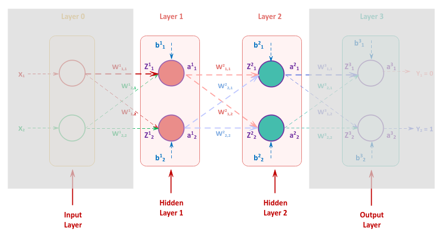
As a result, the gradient of any neuron in the first hidden layer is computed as the sum of gradients from the two neurons in the second hidden layer. In other words, the sum of gradients $\delta_1^2$ and $\delta_2^2$ influence the change in the bias and the weights of the first hidden layer.
Given that we are using a sigmoid activation function for our neural network , we need an utility function to translate the target class into probabilities of those classes during training.
In other words, if the outcome is a $0$, then $Y_1$ has more probability versus $Y_2$. Similarly, if the outcome is a $1$, then $Y_2$ has more probability versus $Y_1$.
The following code snippet shows the implementation of the target to probabilities transformer:
def probabilities_of_target(target):
  prob = [0.05, 0.95]
  if target == 1:
    prob = [0.95, 0.05]
  return prob
We need an utility function to accumulate the totals. The following code snippet shows the implementation of the utility function:
def accumulate_into_total(totals, vals):
  for i in range(len(totals)):
    totals[i] += vals[i]
The following code snippet shows the implementation of a neuron:
class MyNeuron:
  # Initialize bias and weights via bias_weights - the first item (at zero index) is the bias
  def __init__(self, num_inputs, activation='sigmoid', bias_weights=None):
    self.num_inputs = num_inputs
    match activation:
      case 'sigmoid':
        self.activation_func = activation_sigmoid
      case 'step':
        self.activation_func = activation_step
      case _: # Default activation is sigmoid
        self.activation_func = activation_sigmoid
    self.weights = []
    if bias_weights is None:
      self.bias = np.random.random(1)[0]
      for i in range(num_inputs):
        self.weights.append(np.random.random(1)[0])
    else:
      self.bias = bias_weights[0]
      for i in range(num_inputs):
        self.weights.append(bias_weights[i+1])

  def info(self):
    print('--- [ Neuron ] ---')
    print('No. of Inputs:', self.num_inputs)
    print('Bias:', self.bias, ', Weights:', self.weights)

  # Method to compute the weighted sum (z)
  def compute_z(self, row):
    weighted_sum = self.bias
    for i in range(self.num_inputs):
      weighted_sum += (row[i] * self.weights[i])
    return weighted_sum

  # Method to compute the activation (a) for the given weighted sum (z)
  def compute_a(self, z):
    return self.activation_func(z)

  def adjust_weight(self, alpha, dz_dw, delta):
    for i in range(self.num_inputs):
      self.weights[i] -= (alpha * dz_dw[i] * delta)

  def adjust_bias(self, alpha, delta):
      self.bias -= (alpha * delta)
The following code snippet shows the implementation of a layer in the neural network:
class MyNeuralNetworkLayer:
  # Initialize bias and weights of the neuron(s) via weights_list [list of [list]]
  def __init__(self, layer_id, num_inputs, num_neurons, weights_list=None):
    self.layer_id = layer_id
    self.num_inputs = num_inputs
    self.num_neurons = num_neurons
    if weights_list is None:
      self.neurons = [MyNeuron(num_inputs) for _ in range(num_neurons)]
    else:
      self.neurons = [MyNeuron(num_inputs, bias_weights=weights_list[i]) for i in range(num_neurons)]
    self.input_values = [0.0 for _ in range(num_inputs)]
    self.z_values = [0.0 for _ in range(num_neurons)]
    self.a_values = [0.0 for _ in range(num_neurons)]
    self.da_dz_values = [0.0 for _ in range(num_neurons)]
    self.delta_values = [0.0 for _ in range(num_neurons)]

  def info(self):
    print('~~~~~~ [ Layer -', self.layer_id, '] ~~~~~~')
    print('No. of Neurons:', self.num_neurons)
    print('Input:', self.input_values)
    print('Z Values:', self.z_values)
    print('A Values:', self.a_values)
    for neuron in self.neurons:
      neuron.info()

  # Compute the weighted sum (z) and activation (a) values for all neuron(s) in this layer
  def compute_z_and_a(self, row):
    self.input_values = row
    for i in range(self.num_neurons):
      neuron = self.neurons[i]
      z = neuron.compute_z(row)
      a = neuron.compute_a(z)
      self.z_values[i] = z
      self.a_values[i] = a

  def compute_mse_loss(self, actual, size):
    mse_loss = []
    for i in range(len(self.a_values)):
      mse = (self.a_values[i] - actual[i]) ** 2
      mse_loss.append(mse/size)
    return mse_loss

  # Derivative of the loss over the output probabilities
  def compute_dl_da(self, actual, size):
    loss_over_a = []
    for i in range(len(self.a_values)):
      grad = 2.0 * (self.a_values[i] - actual[i])
      loss_over_a.append(grad/size)
    return loss_over_a

  # Derivative of output (activation) over input (weighted sum)
  def compute_da_dz(self):
    for i in range(self.num_neurons):
      self.da_dz_values[i] = self.a_values[i] * (1 - self.a_values[i])
And now for the final piece - the neural network !!!
The following code snippet shows the implementation of a neural network:
class MyNeuralNetwork:
  # Initialize bias & weights of the hidden layers via hidden_weights [list of [list of [list]]]
  #   AND
  # bias & weights of the output layer via output_weights [list of [list]]
  def __init__(self, num_inputs, hidden_layer_sizes, num_outputs, eta=0.05, epoch=100,
               hidden_weights=None, output_weights=None):
    self.num_inputs = num_inputs
    self.hidden_layer_sizes = hidden_layer_sizes
    self.num_outputs = num_outputs
    self.eta = eta
    self.epoch = epoch
    id_num = 1
    prev_size = num_inputs
    self.hidden_layers = []
    for size in hidden_layer_sizes:
      if hidden_weights is None:
        self.hidden_layers.append(MyNeuralNetworkLayer(id_num, prev_size, size))
      else:
        self.hidden_layers.append(MyNeuralNetworkLayer(id_num, prev_size, size, weights_list=hidden_weights[id_num-1]))
      id_num += 1
      prev_size = size
    if output_weights is None:
      self.output_layer = MyNeuralNetworkLayer(id_num, prev_size, num_outputs)
    else:
      self.output_layer = MyNeuralNetworkLayer(id_num, prev_size, num_outputs, weights_list=output_weights)

  def info(self):
    print('========= [ Neural Network ] =========')
    print('Learning Rate (eta):', self.eta)
    print('Maximum Iterations (epoch):', self.epoch)
    print('Hidden Layer Sizes:', self.hidden_layer_sizes)
    for layer in self.hidden_layers:
        layer.info()
    self.output_layer.info()
    print('======================================')

  def feed_forward(self, row):
    data_row = row
    for layer in self.hidden_layers:
      layer.compute_z_and_a(data_row)
      data_row = layer.a_values
    self.output_layer.compute_z_and_a(data_row)

  def back_propagation(self, dl_da):
    # Reset delta values for all the layers
    self.output_layer.delta_values = [0.0 for _ in range(self.output_layer.num_neurons)]
    for i in range(len(self.hidden_layers), 0, -1):
      self.hidden_layers[i-1].delta_values = [0.0 for _ in range(self.hidden_layers[i-1].num_neurons)]
    # Compute delta for output layer
    self.output_layer.compute_da_dz()
    for i in range(self.output_layer.num_neurons):
      # delta = da/dZ * dL/da
      self.output_layer.delta_values[i] = self.output_layer.da_dz_values[i] * dl_da[i]
    # Adjust weights and bias for the output layer
    for i in range(self.output_layer.num_neurons):
      # W_new = W_old - (eta * input * delta), where input is dL/dW = a
      self.output_layer.neurons[i].adjust_weight(self.eta, self.output_layer.input_values,
                                                self.output_layer.delta_values[i])
      # b_new = b_old - (eta * delta)
      self.output_layer.neurons[i].adjust_bias(self.eta, self.output_layer.delta_values[i])
    # Compute delta for hidden layer(s)
    prev_layer = self.output_layer
    for i in range(len(self.hidden_layers), 0, -1):
      self.hidden_layers[i-1].compute_da_dz()
      # For all the neurons in a hidden layer
      for j in range(self.hidden_layers[i-1].num_neurons):
        # Neurons from the previous layer
        for k in range(prev_layer.num_neurons):
          # delta = da/dZ * dZ/da * prev_layer.delta
          da_dz = self.hidden_layers[i-1].da_dz_values[j]
          dz_da = prev_layer.neurons[k].weights[j]
          # Aggregate all deltas from the previous layer
          self.hidden_layers[i-1].delta_values[j] += (da_dz * dz_da * prev_layer.delta_values[k])
      prev_layer = self.hidden_layers[i-1]
    # Adjust bias and weights for each of the neurons in each of the hidden layer(s) walking backwards
    for i in range(len(self.hidden_layers), 0, -1):
      # For all the neurons in a hidden layer
      for j in range(self.hidden_layers[i-1].num_neurons):
        # W_new = W_old - (eta * input * delta)
        self.hidden_layers[i-1].neurons[j].adjust_weight(self.eta, self.hidden_layers[i-1].input_values,
                                                        self.hidden_layers[i-1].delta_values[j])
        # b_new = b_old - (eta * delta)
        self.hidden_layers[i-1].neurons[j].adjust_bias(self.eta, self.hidden_layers[i-1].delta_values[j])

  def fit(self, x_rows, y_rows, debug=False):
    # Repeat for each iteration up to the max (epoch)
    for loop in range(self.epoch):
      total_mse_loss = [0.0 for _ in range(self.output_layer.num_neurons)]
      total_dl_da = [0.0 for _ in range(self.output_layer.num_neurons)]
      # Repeat for each data sample
      sample_size = len(x_rows)
      for i in range(sample_size):
        row = x_rows[i]
        # actual = probabilities of y_rows[i]
        y_target = y_rows[i]
        actual = probabilities_of_target(y_target)
        self.feed_forward(row)
        # Compute the loss and aggregate to total loss
        mse_loss = self.output_layer.compute_mse_loss(actual, 2.0)
        accumulate_into_total(total_mse_loss, mse_loss)
        # Compute the derivative of loss over a-values and aggregate to total
        dl_da = self.output_layer.compute_dl_da(actual, 2.0)
        accumulate_into_total(total_dl_da, dl_da)
      if debug:
        print('*** Iteration:', loop+1, ', Average Loss:', total_mse_loss)
      # Adjust bias and weights using backpropagation
      self.back_propagation(total_dl_da)

  def predict(self, x_rows):
    y_pred = []
    for i in range(len(x_rows)):
      row = x_rows[i]
      self.feed_forward(row)
      y_pred.append(self.output_layer.a_values.index(max(self.output_layer.a_values)))
    return y_pred
The following code snippet shows how to instantiate our neural network class with a single hidden layer and an output layer:
mynn = MyNeuralNetwork(2, [2], 2)
The following code snippet shows how to display the internal state of a neural network class:
mynn.info()
Executing the above code snippet would result in the following typical output:
========= [ Neural Network ] =========
Learning Rate (eta): 0.05
Maximum Iterations (epoch): 100
Hidden Layer Sizes: [2]
~~~~~~ [ Layer - 1 ] ~~~~~~
No. of Neurons: 2
Input: [0.0, 0.0]
Z Values: [0.0, 0.0]
A Values: [0.0, 0.0]
--- [ Neuron ] ---
No. of Inputs: 2
Bias: 0.17152165622510307 , Weights: [0.6852769816973125, 0.8338968626360765]
--- [ Neuron ] ---
No. of Inputs: 2
Bias: 0.3069662196722378 , Weights: [0.8936130796833973, 0.7215438617683047]
~~~~~~ [ Layer - 2 ] ~~~~~~
No. of Neurons: 2
Input: [0.0, 0.0]
Z Values: [0.0, 0.0]
A Values: [0.0, 0.0]
--- [ Neuron ] ---
No. of Inputs: 2
Bias: 0.18993895420479678 , Weights: [0.5542275911247871, 0.3521319540266141]
--- [ Neuron ] ---
No. of Inputs: 2
Bias: 0.18189240266007867 , Weights: [0.7856017618643588, 0.9654832224119693]
======================================
The following code snippet shows how to train our neural network using a sample training data set and then display its internal state:
X = [
  [1.2, 1.6],
  [7.6, 6.8],
  [3.4, 4.4],
  [6.9, 8.8],
  [3.0, 3.2],
  [5.6, 6.8],
  [2.2, 1.8],
  [5.8, 5.2],
  [1.8, 2.2],
  [6.5, 4.8]
]
y = [0, 1, 0, 1, 0, 1, 0, 1, 0, 1]

mynn.fit(X, y)
mynn.info()
Executing the above code snippet would result in the following typical output:
========= [ Neural Network ] =========
Learning Rate (eta): 0.05
Maximum Iterations (epoch): 100
Hidden Layer Sizes: [2]
~~~~~~ [ Layer - 1 ] ~~~~~~
No. of Neurons: 2
Input: [6.5, 4.8]
Z Values: [8.623469870999047, 9.576717036602751]
A Values: [0.9998201971688595, 0.9999306806422639]
--- [ Neuron ] ---
No. of Inputs: 2
Bias: 0.17144536825966872 , Weights: [0.6847811099219888, 0.8335306804019916]
--- [ Neuron ] ---
No. of Inputs: 2
Bias: 0.30693386560411573 , Weights: [0.8934027782406043, 0.7213885622413188]
~~~~~~ [ Layer - 2 ] ~~~~~~
No. of Neurons: 2
Input: [0.9998201971688595, 0.9999306806422639]
Z Values: [0.0032454204158872714, 0.007217342007028449]
A Values: [0.5008113543918223, 0.5018043276694744]
--- [ Neuron ] ---
No. of Inputs: 2
Bias: -0.17443398067742752 , Weights: [0.18992000411213625, -0.012215751817731987]
--- [ Neuron ] ---
No. of Inputs: 2
Bias: -0.46007404797898116 , Weights: [0.14375052049004067, 0.3235612337593173]
======================================
Notice from Output.5 above the adjusted biases and weights post training.
The following code snippet shows how to predict outcomes using our neural network with a sample testing data set and display the prediction outcomes:
X_t = [
  [5.2, 6.2],
  [2.1, 2.0],
  [7.1, 6.5]
]
y_t = [1, 0, 1]

y_p = mynn.predict(X_t)

print('Predicted:', y_p)
print('Actual:', y_t)
Executing the above code snippet would result in the following typical output:
Predicted: [1, 0, 1]
Actual: [1, 0, 1]
Notice from Output.6 above that the predictions match what is expected !!!
Our implementation of the neural network is *HIGHLY* inefficient and not *GENERIC*. This was purely to get a better grasp of the inner workings of the core concepts
References