Figure.1
| PolarSPARC |
Introduction to Deep Learning - Part 7
| Bhaskar S | 07/28/2023 |
Introduction
In Introduction to Deep Learning - Part 6 of this series, we continued our journey with PyTorch, covering the creation, training, and evaluation of a non-linear Binary Classification model.
In this article, we will wrap-up the journey on PyTorch by covering the following topics:
Datasets and DataLoaders
Multi-class Classification
Saving and Loading a Model
Hands-on PyTorch
We will now move onto the next section that is related to handling of data sets in PyTorch. The data in real world if often complex and messy. In order to encapsulate the data complexity from the model training, one would make use of the following two utility classes together to present a cleaner facade:
torch.utils.data.Dataset
torch.utils.data.DataLoader
The class torch.utils.data.Dataset encapsulates the data processing aspects, while the class torch.utils.data.DataLoader behaves like an iterable wrapper over the data set samples.
Datasets and DataLoaders
For the hands-on demonstration, let us generate synthetic multi-class blob data and save it as CSV files (features and labels) in a data directory.
To import the necessary Python module(s), execute the following code snippet:
import numpy as np
import pandas as pd
import matplotlib as mpl
import matplotlib.pyplot as plt
import torch
from pathlib import Path
from sklearn.model_selection import train_test_split
from sklearn.datasets import make_blobs
from torch import nn
from torch.utils.data import Dataset, DataLoader
from torchmetrics import Accuracy
To create the multi-class synthetic data with two features, execute the following code snippet:
num_samples = 1000
centers = [[0.0, 0.0], [-5.0, 2.0], [5.0, 2.0], [5.0, -2.0], [-5.0, -2.0]]
np_Xc, np_yc = make_blobs(num_samples, n_features=2, centers=centers, cluster_std=1.2, random_state=101)
To create the tensor objects for the dataset, execute the following code snippet:
Xcp = torch.tensor(np_Xcp, dtype=torch.float)
ycp = torch.tensor(np_ycp, dtype=torch.float).unsqueeze(dim=1)
To create the training and testing samples, execute the following code snippet:
Xc_train, Xc_test, yc_train, yc_test = train_test_split(Xc, yc, test_size=0.2, random_state=101)
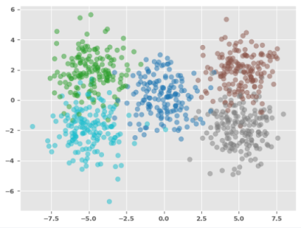
The following illustration shows the plot for the training set:
To define a function to store the training set into a CSV files in the data directory, execute the following code snippet:
def store_training_data(name, X_train, y_train):
  data_path = Path('./data')
  if not data_path.exists():
    data_path.mkdir(exist_ok=True)

  X_path = data_path / Path(name + '-features.csv')
  y_path = data_path / Path(name + '-labels.csv')
  if not X_path.exists():
    df_X = pd.DataFrame(X_train)
    df_y = pd.DataFrame(y_train)
    print(f'---> Storing training features to: {X_path}')
    df_X.to_csv(X_path, index=False)
    print(f'---> Storing training labels to: {y_path}')
    df_y.to_csv(y_path, index=False)
To store the training set in the data directory, execute the following code snippet:
store_training_data('mc-train', Xcp_train, ycp_train)
One would notice two files stored in the data directory - mc-train-features.csv containing the features and mc-train-labels.csv containing the labels.
We will implement a custom torch.utils.data.Dataset class that will load the training set from the two files mc-train-features.csv and mc-train-labels.csv. Note that the custom class MUST implement the following methods:
__init__(self, ...) => runs once when the dataset is instantiated
__len__(self) => returns the number of data samples in the dataset
__getitem__(self, idx) => returns the data sample from the specified index
To define our custom torch.utils.data.Dataset class, execute the following code snippet:
features_tag = 'FEATURES'
target_tag = 'TARGET'

feature_1 = 'X1'
feature_2 = 'X2'
target = 'Y'

class MultiClassDS(Dataset):
  def __init__(self, features_file, labels_file):
    df_X = pd.read_csv(features_file)
    df_X.columns = [feature_1, feature_2]
    df_y = pd.read_csv(labels_file)
    df_y.columns = [target]
    self.features = torch.tensor(df_X.to_numpy(), dtype=torch.float)
    self.target = torch.tensor(df_y.to_numpy(), dtype=torch.long).squeeze(dim=1)

  def __len__(self):
    return len(self.features)

  def __getitem__(self, idx):
    return {features_tag: self.features[idx], target_tag: self.target[idx]}
To test our custom dataset MultiClassDS class, one must access the samples in the dataset via the iterator class torch.utils.data.DataLoader, which provides the flexibility to access the samples in batches with (or without) shuffling.
To create an instance of our custom dataset MultiClassDS and access the samples in batches via the dataloder, execute the following code snippet:
mc_train = MultiClassDS('./data/mc-train-features.csv', './data/mc-train-labels.csv')
train_data = DataLoader(mc_train, batch_size=50, shuffle=False)
for batch in train_data:
  X_mc = batch[features_tag]
  y_mc = batch[target_tag]
  print(f'X_mc Length = {len(X_mc)}, y_mc = {y_mc}')
The following would be a typical output of the first few lines:
X_mc Length = 50, y_mc = tensor([2, 1, 3, 4, 4, 3, 3, 4, 0, 0, 4, 4, 0, 4, 0, 0, 3, 2, 1, 1, 4, 2, 2, 1,
  4, 0, 3, 4, 1, 4, 3, 1, 0, 1, 3, 3, 2, 4, 3, 3, 1, 3, 4, 2, 1, 0, 4, 2,
  3, 3])
X_mc Length = 50, y_mc = tensor([3, 4, 3, 2, 3, 4, 2, 1, 4, 1, 4, 3, 4, 1, 1, 0, 3, 3, 3, 0, 1, 0, 1, 1,
  0, 2, 4, 1, 2, 4, 3, 3, 2, 1, 0, 2, 0, 0, 2, 1, 1, 0, 3, 0, 2, 0, 2, 1,
  2, 3])
X_mc Length = 50, y_mc = tensor([2, 0, 2, 2, 4, 3, 0, 4, 2, 0, 3, 1, 3, 0, 1, 4, 4, 0, 0, 4, 3, 3, 4, 4,
  4, 1, 3, 3, 4, 3, 0, 2, 0, 0, 3, 1, 4, 1, 1, 0, 4, 2, 4, 1, 2, 1, 1, 1,
  2, 0])
X_mc Length = 50, y_mc = tensor([0, 1, 3, 4, 1, 1, 3, 0, 2, 2, 1, 0, 2, 1, 2, 0, 0, 1, 4, 2, 3, 1, 4, 2,
  2, 4, 3, 2, 4, 3, 0, 0, 1, 2, 2, 2, 3, 1, 4, 1, 4, 4, 3, 0, 2, 4, 3, 4,
  0, 2])
...SNIP...
We will now move onto the next section that is related to the loss function associated with a multi-class model.
Softmax Function
In the case of the multi-class classification, we will need some function that would indicate what class the given input would be classified as. This is where the Softmax function comes in handy. It translates the raw output from the neural network into a set of probabilities, where each probability corresponds with a target class.
Given the output $y_i$, the Softmax function $\sigma$ is defined as follows:
$\sigma(y_i) = \Large{\frac{y_i}{\sum_{j=1}^N y_j}}$
where, $N$ is number of target classes and $S(y_i)$ lies in the range $[0, 1]$.
Multi-class Classification Loss Function
In Introduction to Deep Learning - Part 6 of this series, we indicated that for Binary Classification problems, one would use the Binary Cross Entropy loss function.
For Multi-class Classification problems, one would typically use the Cross Entropy loss.
Binary Cross Entropy is a special case of the more generic Cross Entropy loss.
The Cross Entropy loss $L(x, W, b)$ is defined as follows:
$L(x, W, b) = - \sum_{i=1}^N y_i.log(\sigma_i(x, W, b))$
where, $x$ is the input, $W$ is the weights, $b$ is the biases, $\sigma_i$ is the softmax function with its output as the predicted value, and $y_i$ is the actual target prediction class.
We will now move onto the next section that is related to creating, training, and evaluating the multi-class model.
PyTorch Model Basics - Part 3
To define the method to display the decision boundary along with the scatter plot, execute the following code snippet:
def plot_with_decision_boundary(model, X, y):
  margin = 0.1
  # Set the grid bounds - identify min and max values with some margin
  x_min, x_max = X[:, 0].min() - margin, X[:, 0].max() + margin
  y_min, y_max = X[:, 1].min() - margin, X[:, 1].max() + margin
  # Create the x and y scale with spacing
  space = 0.1
  x_scale = np.arange(x_min, x_max, space)
  y_scale = np.arange(y_min, y_max, space)
  # Create the x and y grid
  x_grid, y_grid = np.meshgrid(x_scale, y_scale)
  # Flatten the x and y grid to vectors
  x_flat = x_grid.ravel()
  y_flat = y_grid.ravel()
  # Predict using the model for the combined x and y vectors
  y_p = model(torch.tensor(np.c_[x_flat, y_flat], dtype=torch.float))
  y_p = torch.softmax(y_p, dim=1).argmax(dim=1).numpy()
  y_p = y_p.reshape(x_grid.shape)
  # Plot the contour to display the boundary
  plt.contourf(x_grid, y_grid, y_p, cmap=plt.cm.tab10, alpha=0.3)
  plt.scatter(X[:, 0], X[:, 1], c=y, cmap=plt.cm.tab10, alpha=0.5)
  plt.show()
To initialize variables for the number of features, number of target, number of neurons in a hidden layer, and the maximum number of epochs, execute the following code snippet:
num_features = 2
num_targets = 5
num_hidden = 10
max_epochs = 2001

accuracy = Accuracy(task='multiclass', num_classes=num_targets)
To create a custom class for our Multi Class Classification model without any hidden layers, execute the following code snippet:
class MultiClassModel(nn.Module):
  def __init__(self):
    super(MultiClassModel, self).__init__()
    self.nn_layers = nn.Sequential(
      nn.Linear(num_features, num_targets),
      nn.ReLU()
    )

  def forward(self, cx: torch.Tensor) -> torch.Tensor:
    return self.nn_layers(cx)
To create an instance of MultiClassModel, execute the following code snippet:
mc_model = MultiClassModel()
To create an instance of the cross entropy loss, execute the following code snippet:
mc_criterion = nn.CrossEntropyLoss()
To create an instance of the gradient descent optimizer, execute the following code snippet:
mc_optimizer = torch.optim.SGD(mc_model.parameters(), lr=0.05)
To implement the iterative training loop for the forward pass to predict, compute the loss, and execute the backward pass to adjust the parameters, execute the following code snippet:
for epoch in range(1, max_epochs):
  loss = 0.0
  for batch in train_data:
    X_mc_train = batch[features_tag]
    y_mc_train = batch[target_tag]
    mc_model.train()
    mc_optimizer.zero_grad()
    ymc_logits = mc_model(X_mc_train)
    ymc_predict = torch.softmax(ymc_logits, dim=1).argmax(dim=1)
    loss = mc_criterion(ymc_logits, y_mc_train)
    loss.backward()
    mc_optimizer.step()
  if epoch % 200 == 0:
    print(f'Multi Class Model [1] -> Epoch: {epoch}, Loss: {loss}')
The following would be a typical output:
Multi Class Model [1] -> Epoch: 200, Loss: 0.4883924722671509
Multi Class Model [1] -> Epoch: 400, Loss: 0.47102999687194824
Multi Class Model [1] -> Epoch: 600, Loss: 0.4639538824558258
Multi Class Model [1] -> Epoch: 800, Loss: 0.46006831526756287
Multi Class Model [1] -> Epoch: 1000, Loss: 0.4578549861907959
Multi Class Model [1] -> Epoch: 1200, Loss: 0.4549277126789093
Multi Class Model [1] -> Epoch: 1400, Loss: 0.4528881013393402
Multi Class Model [1] -> Epoch: 1600, Loss: 0.451716810464859
Multi Class Model [1] -> Epoch: 1800, Loss: 0.4493400454521179
Multi Class Model [1] -> Epoch: 2000, Loss: 0.44793567061424255
To predict the target classes using the trained model, execute the following code snippet:
mc_model.eval()
with torch.no_grad():
  ymc_logits_test = mc_model(Xcp_test)
  ymc_predict_test = torch.softmax(ymc_logits_test, dim=1).argmax(dim=1)
To display the model prediction accuracy, execute the following code snippet:
print(f'Multi Class Model [1] -> Accuracy: {accuracy(ymc_predict_test, ycp_test)}')
The following would be a typical output:
Multi Class Model [1] -> Accuracy: 0.7649999856948853
To plot the decision boundary along with the scatter plot using the model, execute the following code snippet:
mc_model.eval()
with torch.no_grad():
  plot_with_decision_boundary(mc_model, Xcp_train, ycp_train)
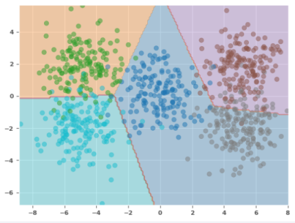
The following illustration depicts the scatter plot with the decision boundary as predicted by the model:
Let us see if we can improve the model by adding a hidden layer.
To create a Multi-class Classification model with one hidden layer consisting of 10 neurons, execute the following code snippet:
class MultiClassModel_2(nn.Module):
  def __init__(self):
    super(MultiClassModel_2, self).__init__()
    self.nn_layers = nn.Sequential(
      nn.Linear(num_features, num_hidden),
      nn.ReLU(),
      nn.Linear(num_hidden, num_targets),
      nn.ReLU()
    )

  def forward(self, cx: torch.Tensor) -> torch.Tensor:
    return self.nn_layers(cx)
To create an instance of MultiClassModel_2, execute the following code snippet:
mc_model_2 = MultiClassModel_2()
To create an instance of the loss function, execute the following code snippet:
mc_criterion_2 = nn.CrossEntropyLoss()
To create an instance of the gradient descent optimizer, execute the following code snippet:
mc_optimizer_2 = torch.optim.SGD(mc_model_2.parameters(), lr=0.05)
To implement the iterative training loop for the forward pass to predict, compute the loss, and execute the backward pass to adjust the parameters, execute the following code snippet:
for epoch in range(1, max_epochs):
  loss = 0.0
  for batch in train_data:
    X_mc_train = batch[features_tag]
    y_mc_train = batch[target_tag]
    mc_model_2.train()
    mc_optimizer_2.zero_grad()
    ymc_logits = mc_model_2(X_mc_train)
    ymc_predict = torch.softmax(ymc_logits, dim=1).argmax(dim=1)
    loss = mc_criterion_2(ymc_logits, y_mc_train)
    loss.backward()
    mc_optimizer_2.step()
  if epoch % 200 == 0:
    print(f'Multi Class Model [2] -> Epoch: {epoch}, Loss: {loss}')
The following would be a typical output:
Multi Class Model [2] -> Epoch: 200, Loss: 0.19411079585552216
Multi Class Model [2] -> Epoch: 400, Loss: 0.18489240109920502
Multi Class Model [2] -> Epoch: 600, Loss: 0.1810990869998932
Multi Class Model [2] -> Epoch: 800, Loss: 0.1787499040365219
Multi Class Model [2] -> Epoch: 1000, Loss: 0.17727196216583252
Multi Class Model [2] -> Epoch: 1200, Loss: 0.17635422945022583
Multi Class Model [2] -> Epoch: 1400, Loss: 0.17572957277297974
Multi Class Model [2] -> Epoch: 1600, Loss: 0.17534948885440826
Multi Class Model [2] -> Epoch: 1800, Loss: 0.17489103972911835
Multi Class Model [2] -> Epoch: 2000, Loss: 0.1745576709508896
To predict the target classes using the trained model, execute the following code snippet:
mc_model_2.eval()
with torch.no_grad():
  y_probabilities_test_2 = mc_model_2(Xcp_test)
  ycp_predict_test_2 = torch.softmax(y_probabilities_test_2, dim=1).argmax(dim=1)
To display the model prediction accuracy, execute the following code snippet:
print(f'Multi Class Model [2] -> Accuracy: {accuracy(ycp_predict_test_2, ycp_test)}')
The following would be a typical output:
Multi Class Model [2] -> Accuracy: 0.8999999761581421
To plot the decision boundary along with the scatter plot using the model, execute the following code snippet:
mc_model_2.eval()
with torch.no_grad():
  plot_with_decision_boundary(mc_model_2, Xcp_train, ycp_train)
The following illustration depicts the scatter plot with the decision boundary as predicted by the model:
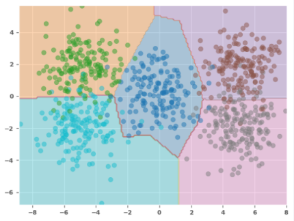
The prediction accuracy has improved a little bit. Also, we observe a better demarcation between the classes from the plot in Figure.3 above.
One last time, let us see if we can improve the model by adding one more hidden layer for a total of two.
To create a Multi-class Classification model with two hidden layers - the first and the second hidden layer each consisting of 10 neurons, execute the following code snippet:
class MultiClassModel_3(nn.Module):
  def __init__(self):
    super(MultiClassModel_3, self).__init__()
    self.nn_layers = nn.Sequential(
      nn.Linear(num_features, num_hidden),
      nn.ReLU(),
      nn.Linear(num_hidden, num_hidden),
      nn.ReLU(),
      nn.Linear(num_hidden, num_targets),
      nn.ReLU()
    )

  def forward(self, cx: torch.Tensor) -> torch.Tensor:
    return self.nn_layers(cx)
To create an instance of MultiClassModel_3, execute the following code snippet:
mc_model_3 = MultiClassModel_3()
To create an instance of the loss function, execute the following code snippet:
mc_criterion_3 = nn.CrossEntropyLoss()
To create an instance of the gradient descent optimizer, execute the following code snippet:
mc_optimizer_3 = torch.optim.SGD(mc_model_3.parameters(), lr=0.05)
To implement the iterative training loop for the forward pass to predict, compute the loss, and execute the backward pass to adjust the parameters, execute the following code snippet:
for epoch in range(1, max_epochs):
  loss = 0.0
  for batch in train_data:
    X_mc_train = batch[features_tag]
    y_mc_train = batch[target_tag]
    mc_model_3.train()
    mc_optimizer_3.zero_grad()
    ymc_logits = mc_model_3(X_mc_train)
    ymc_predict = torch.softmax(ymc_logits, dim=1).argmax(dim=1)
    loss = mc_criterion_3(ymc_logits, y_mc_train)
    loss.backward()
    mc_optimizer_3.step()
  if epoch % 200 == 0:
    print(f'Multi Class Model [3] -> Epoch: {epoch}, Loss: {loss}')
The following would be a typical output:
Multi Class Model [3] -> Epoch: 200, Loss: 0.7063612937927246
Multi Class Model [3] -> Epoch: 400, Loss: 0.7020133137702942
Multi Class Model [3] -> Epoch: 600, Loss: 0.6979369521141052
Multi Class Model [3] -> Epoch: 800, Loss: 0.6961963176727295
Multi Class Model [3] -> Epoch: 1000, Loss: 0.6950473189353943
Multi Class Model [3] -> Epoch: 1200, Loss: 0.6934585571289062
Multi Class Model [3] -> Epoch: 1400, Loss: 0.6918855309486389
Multi Class Model [3] -> Epoch: 1600, Loss: 0.6914334893226624
Multi Class Model [3] -> Epoch: 1800, Loss: 0.6915342211723328
Multi Class Model [3] -> Epoch: 2000, Loss: 0.6914027333259583
To predict the target classes using the trained model, execute the following code snippet:
mc_model_3.eval()
with torch.no_grad():
  y_probabilities_test_3 = mc_model_3(Xcp_test)
  ycp_predict_test_3 = torch.softmax(y_probabilities_test_3, dim=1).argmax(dim=1)
To display the model prediction accuracy, execute the following code snippet:
print(f'Multi Class Model [3] -> Accuracy: {accuracy(ycp_predict_test_3, ycp_test)}')
The following would be a typical output:
Multi Class Model [3] -> Accuracy: 0.7450000047683716
From the Output.7 above, we see a poorer performing model !!!
To plot the decision boundary along with the scatter plot using the model, execute the following code snippet:
mc_model_3.eval()
with torch.no_grad():
  plot_with_decision_boundary(mc_model_3, Xcp_train, ycp_train)
The following illustration depicts the scatter plot with the decision boundary as predicted by the model:
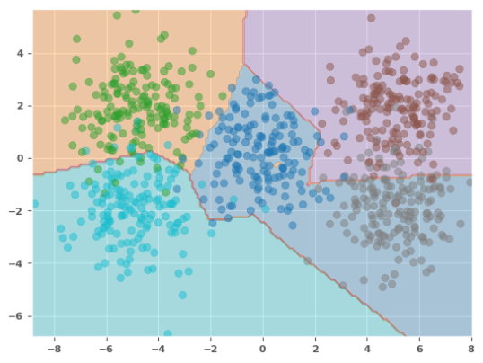
From the plot in Figure.4 above, we see the decision boundaries are messed up. Adding more layers has CLEARLY not helped in this case !!!
Finally, onto the section that is related to saving, loading, and evaluating the loaded multi-class model.
Saving and Loading Model
To save the state of the trained model in the ./models directory, execute the following code snippet:
model_path = './models'
model_state_file = './models/mc-model2-state.pth'

if not Path(model_path).exists():
  Path(model_path).mkdir(exist_ok=True)

# Always save
torch.save(mc_model_2.state_dict(), f=model_state_file)
One would notice a file stored in the models directory - mc-model2-state.pth containing the the state (parameters) of the second model.
To load the state of the trained model from the models directory and evaluate the loaded model, execute the following code snippet:
mc_model_2_new = MultiClassModel_2()
mc_model_2_new.load_state_dict(torch.load(f=model_state_file))
mc_model_2_new.eval()
with torch.no_grad():
  y_probabilities_test_4 = mc_model_2_new(Xcp_test)
  ycp_predict_test_4 = torch.softmax(y_probabilities_test_4, dim=1).argmax(dim=1)
To display the prediction accuracy of the loaded model, execute the following code snippet:
print(f'Loaded Multi Class Model [4] -> Accuracy: {accuracy(ycp_predict_test_4, ycp_test)}')
The following would be a typical output:
Loaded Multi Class Model [4] -> Accuracy: 0.8999999761581421
The result from Output.8 matches the result from Output.5 above.
References
Introduction to Deep Learning - Part 6
Introduction to Deep Learning - Part 5
Introduction to Deep Learning - Part 4
Introduction to Deep Learning - Part 3