Figure.1
| PolarSPARC |
Introduction to Deep Learning - Part 6
| Bhaskar S | 07/22/2023 |
Introduction
In Introduction to Deep Learning - Part 5 of this series, we continued our journey with PyTorch, covering the following topics:
Tensor Shape Manipulation
Autograd Feature
Building Basic Linear Models (with and without GPU)
In this article, we will continue the journey further in building a non-linear PyTorch model.
Hands-on PyTorch
We will now move onto the next section on building a non-linear Binary Classification model.
Binary Classification Loss Function
In Introduction to Deep Learning - Part 2 of this series, we described the Loss Function as a measure of the deviation of the predicted value from the actual target value.
For Regression problems, one would either use the Mean Absolute Error (also known as the L1 Loss) or the Mean Squared Error loss.
However, for Classification problems, one would typically use the Cross Entropy loss, in particular the Binary Cross Entropy loss for the Binary Classification problems.
The Binary Cross Entropy loss $L(x, W, b)$ is defined as follows:
$L(x, W, b) = -[y.log(\sigma(x, W, b)) + (1 - y).log(1-\sigma(x, W, b))]$
where, $x$ is the input, $W$ is the weights, $b$ is the biases, $\sigma$ is the activation function with its output as the predicted value, and $y$ is the actual target prediction class.
PyTorch Model Basics - Part 2
For the non-linear Binary Classification use-case, we will leverage one of the Scikit-Learn capabilities to create the non-linear synthetic data.
To import the necessary Python module(s), execute the following code snippet:
import numpy as np
import matplotlib.pyplot as plt
from sklearn.model_selection import train_test_split
from sklearn.datasets import make_moons
from sklearn.metrics import accuracy_score
import torch
from torch import nn
To create the non-linear synthetic data for the Binary Classification with two features, execute the following code snippet:
num_samples = 500

np_Xcp, np_ycp = make_moons(num_samples, noise=0.15, random_state=101)
To create the tensor dataset, execute the following code snippet:
Xcp = torch.tensor(np_Xcp, dtype=torch.float)
ycp = torch.tensor(np_ycp, dtype=torch.float).unsqueeze(dim=1)
To create the training and testing samples, execute the following code snippet:
Xc_train, Xc_test, yc_train, yc_test = train_test_split(Xc, yc, test_size=0.2, random_state=101)
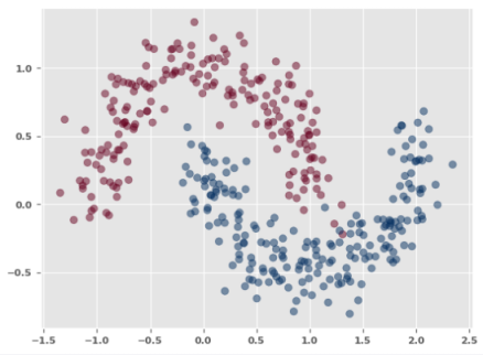
The following illustration shows the plot for the training set:
To initialize variables for the number of features, number of target, and the number of epoch, execute the following code snippet:
num_features_3 = 2
num_target_3 = 1
num_epochs_3 = 2001
To create a simple non-linear Binary Classification model without any hidden layers for the above case, execute the following code snippet:
class BinaryClassNonLinearModel(nn.Module):
  def __init__(self):
    super(BinaryClassNonLinearModel, self).__init__()
    self.nn_layers = nn.Sequential(
      nn.Linear(num_features_3, num_target_3),
      nn.Sigmoid()
    )

  def forward(self, cx: torch.Tensor) -> torch.Tensor:
    return self.nn_layers(cx)
To create an instance of BinaryClassNonLinearModel, execute the following code snippet:
nl_model = BinaryClassNonLinearModel()
To create an instance of the Binary Cross Entropy loss function, execute the following code snippet:
nl_criterion = nn.BCELoss()
To create an instance of the gradient descent function, execute the following code snippet:
nl_optimizer = torch.optim.SGD(nl_model.parameters(), lr=0.05)
To implement the iterative training loop for the forward pass to predict, compute the loss, and execute the backward pass to adjust the parameters, execute the following code snippet:
for epoch in range(1, num_epochs_3):
  nl_model.train()
  nl_optimizer.zero_grad()
  ycp_predict = nl_model(Xcp_train)
  loss = nl_criterion(ycp_predict, ycp_train)
  if epoch % 100 == 0:
    print(f'Non-Linear Model [1] -> Epoch: {epoch}, Loss: {loss}')
  loss.backward()
  nl_optimizer.step()
The following would be a typical output:
Non-Linear Model [1] -> Epoch: 100, Loss: 0.4583107829093933
Non-Linear Model [1] -> Epoch: 200, Loss: 0.38705599308013916
Non-Linear Model [1] -> Epoch: 300, Loss: 0.35396769642829895
Non-Linear Model [1] -> Epoch: 400, Loss: 0.333740770816803
Non-Linear Model [1] -> Epoch: 500, Loss: 0.3197369873523712
Non-Linear Model [1] -> Epoch: 600, Loss: 0.3093145191669464
Non-Linear Model [1] -> Epoch: 700, Loss: 0.30119335651397705
Non-Linear Model [1] -> Epoch: 800, Loss: 0.29466748237609863
Non-Linear Model [1] -> Epoch: 900, Loss: 0.2893083989620209
Non-Linear Model [1] -> Epoch: 1000, Loss: 0.2848363220691681
Non-Linear Model [1] -> Epoch: 1100, Loss: 0.28105801343917847
Non-Linear Model [1] -> Epoch: 1200, Loss: 0.27783405780792236
Non-Linear Model [1] -> Epoch: 1300, Loss: 0.27506041526794434
Non-Linear Model [1] -> Epoch: 1400, Loss: 0.2726573050022125
Non-Linear Model [1] -> Epoch: 1500, Loss: 0.2705625891685486
Non-Linear Model [1] -> Epoch: 1600, Loss: 0.26872673630714417
Non-Linear Model [1] -> Epoch: 1700, Loss: 0.2671099007129669
Non-Linear Model [1] -> Epoch: 1800, Loss: 0.26567962765693665
Non-Linear Model [1] -> Epoch: 1900, Loss: 0.2644093632698059
Non-Linear Model [1] -> Epoch: 2000, Loss: 0.26327699422836304
To predict the target values using the trained model, execute the following code snippet:
nl_model.eval()
with torch.no_grad():
  y_predict_nl = nl_model(Xcp_test)
  y_predict_nl = torch.round(y_predict_nl)
To display the model prediction accuracy, execute the following code snippet:
print(f'Non-Linear Model [1] -> Accuracy: {accuracy_score(y_predict_nl, ycp_test)}')
The following would be a typical output:
Non-Linear Model [1] -> Accuracy: 0.86
A visual plot of the decision boundary that segregates the two classes would be very useful.
To define the method to display the decision boundary along with the scatter plot, execute the following code snippet:
def plot_with_decision_boundary(model, X, y):
  margin = 0.1
  # Set the grid bounds - identify min and max values with some margin
  x_min, x_max = X[:, 0].min() - margin, X[:, 0].max() + margin
  y_min, y_max = X[:, 1].min() - margin, X[:, 1].max() + margin
  # Create the x and y scale with spacing
  space = 0.1
  x_scale = np.arange(x_min, x_max, space)
  y_scale = np.arange(y_min, y_max, space)
  # Create the x and y grid
  x_grid, y_grid = np.meshgrid(x_scale, y_scale)
  # Flatten the x and y grid to vectors
  x_flat = x_grid.ravel()
  y_flat = y_grid.ravel()
  # Predict using the model for the combined x and y vectors
  y_p = model(torch.tensor(np.c_[x_flat, y_flat], dtype=torch.float)).numpy()
  y_p = y_p.reshape(x_grid.shape)
  # Plot the contour to display the boundary
  plt.contourf(x_grid, y_grid, y_p, cmap=plt.cm.RdBu, alpha=0.3)
  plt.scatter(X[:, 0], X[:, 1], c=y, cmap=plt.cm.RdBu, alpha=0.5)
  plt.show()
To plot the decision boundary along with the scatter plot on the training data using the model we just created above, execute the following code snippet:
nl_model.eval()
with torch.no_grad():
  plot_with_decision_boundary(nl_model, Xcp_train, ycp_train)
The following illustration depicts the scatter plot with the decision boundary as predicted by the model:
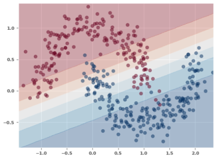
Given that the model uses a linear layer it is not surprising to see a linear demarcation between the two classes from the plot in Figure.2 above.
Let us see if we can improve the model by adding a hidden layer.
To create a non-linear Binary Classification model with one hidden layer consisting of 8 neurons, execute the following code snippet:
num_hidden_3 = 8

class BinaryClassNonLinearModel_2(nn.Module):
  def __init__(self):
    super(BinaryClassNonLinearModel_2, self).__init__()
    self.nn_layers = nn.Sequential(
      nn.Linear(num_features_3, num_hidden_3),
      nn.ReLU(),
      nn.Linear(num_hidden_3, num_target_3),
      nn.Sigmoid()
    )

  def forward(self, cx: torch.Tensor) -> torch.Tensor:
    return self.nn_layers(cx)
To create an instance of BinaryClassNonLinearModel_2, execute the following code snippet:
nl_model_2 = BinaryClassNonLinearModel_2()
To create an instance of the Binary Cross Entropy loss function, execute the following code snippet:
nl_criterion_2 = nn.BCELoss()
To create an instance of the gradient descent function, execute the following code snippet:
nl_optimizer_2 = torch.optim.SGD(nl_model_2.parameters(), lr=0.05)
To implement the iterative training loop for the forward pass to predict, compute the loss, and execute the backward pass to adjust the parameters, execute the following code snippet:
for epoch in range(1, num_epochs_3):
  nl_model_2.train()
  nl_optimizer_2.zero_grad()
  ycp_predict = nl_model_2(Xcp_train)
  loss = nl_criterion_2(ycp_predict, ycp_train)
  if epoch % 100 == 0:
    print(f'Non-Linear Model [2] -> Epoch: {epoch}, Loss: {loss}')
  loss.backward()
  nl_optimizer_2.step()
The following would be a typical output:
Non-Linear Model [2] -> Epoch: 200, Loss: 0.3945632874965668
Non-Linear Model [2] -> Epoch: 300, Loss: 0.33575549721717834
Non-Linear Model [2] -> Epoch: 400, Loss: 0.3044913411140442
Non-Linear Model [2] -> Epoch: 500, Loss: 0.2857321798801422
Non-Linear Model [2] -> Epoch: 600, Loss: 0.27366170287132263
Non-Linear Model [2] -> Epoch: 700, Loss: 0.26533225178718567
Non-Linear Model [2] -> Epoch: 800, Loss: 0.2591221332550049
Non-Linear Model [2] -> Epoch: 900, Loss: 0.2543095052242279
Non-Linear Model [2] -> Epoch: 1000, Loss: 0.2502143681049347
Non-Linear Model [2] -> Epoch: 1100, Loss: 0.24629908800125122
Non-Linear Model [2] -> Epoch: 1200, Loss: 0.24235355854034424
Non-Linear Model [2] -> Epoch: 1300, Loss: 0.23860971629619598
Non-Linear Model [2] -> Epoch: 1400, Loss: 0.23535583913326263
Non-Linear Model [2] -> Epoch: 1500, Loss: 0.23240886628627777
Non-Linear Model [2] -> Epoch: 1600, Loss: 0.2295774221420288
Non-Linear Model [2] -> Epoch: 1700, Loss: 0.22672024369239807
Non-Linear Model [2] -> Epoch: 1800, Loss: 0.2237909436225891
Non-Linear Model [2] -> Epoch: 1900, Loss: 0.22083352506160736
Non-Linear Model [2] -> Epoch: 2000, Loss: 0.21780216693878174
To predict the target values using the trained model, execute the following code snippet:
nl_model_2.eval()
with torch.no_grad():
  y_predict_nl_2 = nl_model_2(Xcp_test)
  y_predict_nl_2 = torch.round(y_predict_nl_2)
To display the model prediction accuracy, execute the following code snippet:
print(f'Non-Linear Model [2] -> Accuracy: {accuracy_score(y_predict_nl_2, ycp_test)}')
The following would be a typical output:
Non-Linear Model [2] -> Accuracy: 0.89
To plot the decision boundary along with the scatter plot on the training data using the model we just created above, execute the following code snippet:
nl_model_2.eval()
with torch.no_grad():
  plot_with_decision_boundary(nl_model_2, Xcp_train, ycp_train)
The following illustration depicts the scatter plot with the decision boundary as predicted by the model:
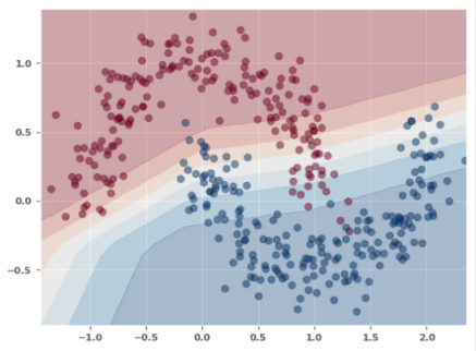
The prediction accuracy has improved a little bit. Also, we observe a better demarcation between the two classes from the plot in Figure.3 above.
One last time, let us see if we can improve the model by adding one more hidden layer for a total of two.
To create a non-linear Binary Classification model with two hidden layers - the first hidden layer consisting of 16 neurons and the second hidden layer consisting of 8 neurons, execute the following code snippet:
num_hidden_1_3 = 16
num_hidden_2_3 = 8

class BinaryClassNonLinearModel_3(nn.Module):
  def __init__(self):
    super(BinaryClassNonLinearModel_3, self).__init__()
    self.hidden_layer = nn.Sequential(
      nn.Linear(num_features_3, num_hidden_1_3),
      nn.ReLU(),
      nn.Linear(num_hidden_1_3, num_hidden_2_3),
      nn.ReLU(),
      nn.Linear(num_hidden_2_3, num_target_3),
      nn.Sigmoid()
    )

  def forward(self, cx: torch.Tensor) -> torch.Tensor:
    return self.hidden_layer(cx)
To create an instance of BinaryClassNonLinearModel_3, execute the following code snippet:
nl_model_3 = BinaryClassNonLinearModel_3()
To create an instance of the Binary Cross Entropy loss function, execute the following code snippet:
nl_criterion_3 = nn.BCELoss()
To create an instance of the gradient descent function, execute the following code snippet:
nl_optimizer_3 = torch.optim.SGD(nl_model_3.parameters(), lr=0.05)
To implement the iterative training loop for the forward pass to predict, compute the loss, and execute the backward pass to adjust the parameters, execute the following code snippet:
for epoch in range(1, num_epochs_3):
  nl_model_3.train()
  nl_optimizer_3.zero_grad()
  ycp_predict = nl_model_3(Xcp_train)
  loss = nl_criterion_3(ycp_predict, ycp_train)
  if epoch % 100 == 0:
    print(f'Non-Linear Model [3] -> Epoch: {epoch}, Loss: {loss}')
  loss.backward()
  nl_optimizer_3.step()
The following would be a typical output:
Non-Linear Model [3] -> Epoch: 200, Loss: 0.32728901505470276
Non-Linear Model [3] -> Epoch: 300, Loss: 0.26362675428390503
Non-Linear Model [3] -> Epoch: 400, Loss: 0.2460920661687851
Non-Linear Model [3] -> Epoch: 500, Loss: 0.23748859763145447
Non-Linear Model [3] -> Epoch: 600, Loss: 0.22980321943759918
Non-Linear Model [3] -> Epoch: 700, Loss: 0.2213612049818039
Non-Linear Model [3] -> Epoch: 800, Loss: 0.21136374771595
Non-Linear Model [3] -> Epoch: 900, Loss: 0.1993836611509323
Non-Linear Model [3] -> Epoch: 1000, Loss: 0.1850656270980835
Non-Linear Model [3] -> Epoch: 1100, Loss: 0.1690329909324646
Non-Linear Model [3] -> Epoch: 1200, Loss: 0.15195232629776
Non-Linear Model [3] -> Epoch: 1300, Loss: 0.1345341056585312
Non-Linear Model [3] -> Epoch: 1400, Loss: 0.1175856664776802
Non-Linear Model [3] -> Epoch: 1500, Loss: 0.10193011909723282
Non-Linear Model [3] -> Epoch: 1600, Loss: 0.08826065808534622
Non-Linear Model [3] -> Epoch: 1700, Loss: 0.07683814316987991
Non-Linear Model [3] -> Epoch: 1800, Loss: 0.06754428148269653
Non-Linear Model [3] -> Epoch: 1900, Loss: 0.060103677213191986
Non-Linear Model [3] -> Epoch: 2000, Loss: 0.05398537218570709
From the Output.5 above, we see the loss reduce quite a bit, which is great !!!
To predict the target values using the trained model, execute the following code snippet:
nl_model_3.eval()
with torch.no_grad():
  y_predict_nl_3 = nl_model_3(Xcp_test)
  y_predict_nl_3 = torch.round(y_predict_nl_3)
To display the model prediction accuracy, execute the following code snippet:
print(f'Non-Linear Model [3] -> Accuracy: {accuracy_score(y_predict_nl_3, ycp_test)}')
The following would be a typical output:
Non-Linear Model [3] -> Accuracy: 0.96
From the Output.6 above, we clearly see a BETTER performing model.
To plot the decision boundary along with the scatter plot on the training data using the model we just created above, execute the following code snippet:
nl_model_3.eval()
with torch.no_grad():
  plot_with_decision_boundary(nl_model_3, Xcp_train, ycp_train)
The following illustration depicts the scatter plot with the decision boundary as predicted by the model:
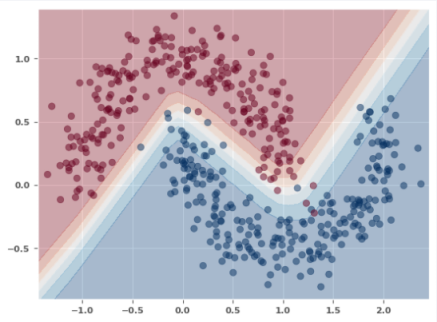
WALLA !!! We observe a much better demarcation between the two classes from the plot in Figure.4 above.
References
Introduction to Deep Learning - Part 5
Introduction to Deep Learning - Part 4
Introduction to Deep Learning - Part 3