Figure.1
| PolarSPARC |
Deep Learning - Understanding the Transformer Models
| Bhaskar S | 12/10/2023 |
Introduction
Of late, there is a lot of BUZZ around Large Language Models (or LLMs for short) with the release of ChatGPT from OpenAI. In short, ChatGPT is an advanced form of a ChatBot that engages in any type of conversation with the users (referred to as Conversational AI).
In the article Deep Learning - Sequence-to-Sequence Model, we introduced the concept of the Encoder-Decoder model for language translation. The same model can also be used to accomplish the task of a ChatBot. So what is all the excitement around the LLM models (aka ChatGPT) ???
Given that the amount of data from the Internet is in ZETTABYTES, there are two challenges with the Seq2Seq model:
It will not be able to retain all the contextual information for such vast amounts of data
It will be super SLOW to train, given it deals with one word at a time
To address these challenges, Google published the Attention Is All You Need paper in 2017, which led to the creation of the next breed of language model called the Transformer model.
In this article, we will unravel the mystery behind Transformer models, so we have a better intuition of how they work.
Inside the Transformer Model
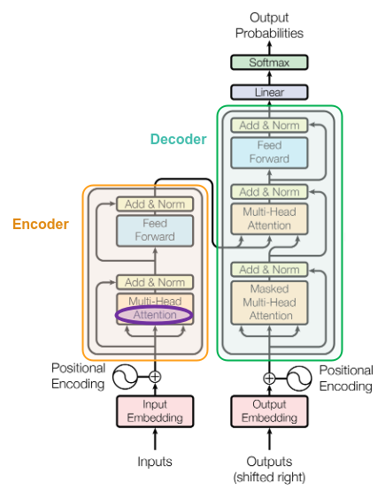
The following illustration shows the architecture of a Transformer model from the paper:
A Transformer model has the Encoder and the Decoder blocks similar to the Seq2Seq model, with the ability to process all the words in a given sentence in parallel (versus sequentially one at a time). However, the most CRUCIAL block is the one highlighted in purple in Figure.1 above - Attention (also referred to as Self-Attention).
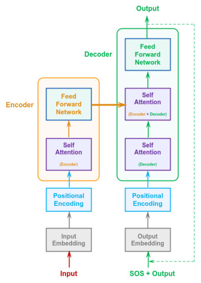
For better understanding, we will simplify the architecture shown in Figure.1 above to the one as shown below:
To get an intuition on Attention, let us consider the following two sentences:
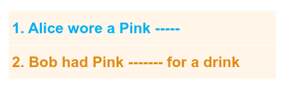
A human brain can look at the two sentences in Figure.3 above and quickly fill in the word dress for sentence 1 and the word Lemonade for sentence 2.
How is the human brain able to do this ???
For sentence 1, the human brain focussed or paid attention to the word wore to guess the missing word as dress.
Similarly, for sentence 2, the human brain paid attention to the word drink to guess the missing word as Lemonade.
In other words, the human brain is able to selectively focus on some words in a sentence to figure the context of the sentence and fill in the blanks. Intuitively, this is how the human Attention mechanism works.
Let us look at another longer sentence as shown below:
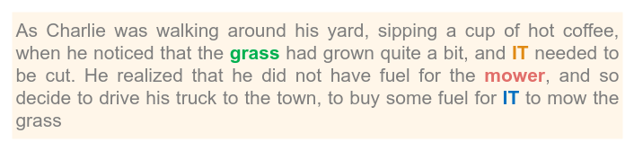
There are two IT in the long sentence above. What are they referring to ???
The human brain very quickly will be able to associate the first IT with the word grass and the second IT with the word mower.
Given the longer sentence, the human brain pays attention to only few words to determine the context and relationships between words.
In the Seq2Seq model, every word is processed irrespective of its importance. This is one of the reasons, why it performed poorly with large text corpus.
But, how do we mimic the attention mechanism like the human brain in a neural network ???
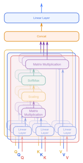
From the paper, how Attention can be computed is shown using the following illustration:
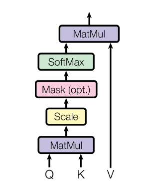
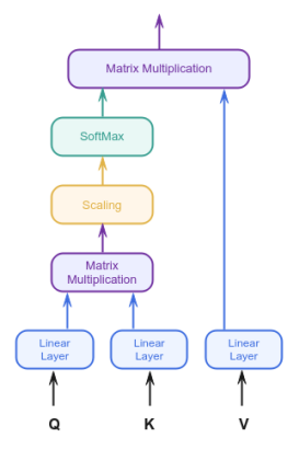
For clarity, we will redraw the Attention block shown in Figure.5 above with the following simplified illustration:
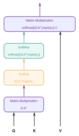
In mathematical terms, the Attention is computed as follows:
$Attention(Q, K, V) = softmax(\Large{\frac{Q.K^T}{\sqrt{d_k}}})\normalsize{.V}$
Let us unravel and understand the Attention mechanism computation from Figure.6 above.
As hinted above, the human brain tries to find the relationships and similarities between words and determine the context of a sentence based on STRONG similarities. This is where the aid of Word Embeddings and Word Similarities come in handy.
In the article Deep Learning - Word Embeddings with Word2Vec, we introduced the concept of Word Embeddings and the use of the Vector Dot Product to determine the closeness or similarity between words. In short, when two words are similar to each other in meaning or relationship, the dot product of their embeddings will be greater than zero.
The question one may have at this point - how does the dot product of the embeddings mimic attention mechanism ???
To explain the computation of Attention, let us consider the following simple sentence:
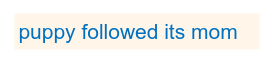
The matrices $Q$, $K$, and $V$ are all the SAME and nothing more than the word embedding vector for each of the words in the sentence stacked as rows, as shown in the illustration below:
Note that we have arbitrarily chose a word embedding of size $4$ and arbitrarily assigned the values for the corresponding word embedding vector.
The first step in finding Attention is to compute the dot product $Q.K^T$. What this is trying to determine is how similar are each of the words to the other words in the sentence.
In other words, for each word $q_i$ from the matrix $Q$ (represents all the words of the sentence), we are finding the word similarity with each of the words $k_j$ from the matrix $K$ (representation of all the words from the sentence). Rather than performing the operations in this sequential manner, we are using the matrix representation $Q.K^T$ for efficiency (vectorized operation).
One way to think of this - it is similar to making a QUERY (hence represented as $Q$) with all the KEYS (hence represented as $K$) to determine how similar each of the words are and returning a vector of scores. The result of this operation is what is referred to as the Similarity Scores (or Attention Scores).
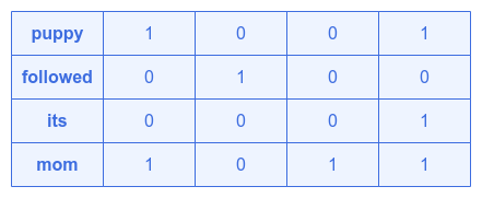
The following illustration depicts the outcome of the dot product $Q.K^T$.:
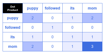
Note that the higher values indicate more similarity between words and hence depicted in darker shades.
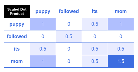
The second step is to normalize or scale the Attention Scores. Note that a typical word embedding vector is at a minimum of size $64$ elements and hence the dot product values tend be large. During the model training, large values have a negative impact on backpropagation (gradient computations) and hence need to be normalized or scaled. Per the paper, the scaling must be done by a factor, which is the $SquareRoot(vector\ size)$. In our example, the vector size is $4$ and hence the scaling factor of $2$.
The following illustration depicts the outcome of the scaled dot product $\Large{\frac{Q.K^T} {\sqrt{d_k}}}$:
The third step is to normalize the Attention Scores to be all positive numbers in the range of $[0, 1]$. Note that we did not pick any negative numbers for our arbitrary word embedding vectors. In the real world, however, the embedding vectors do include negative numbers as well. In order to normalize all the positive/negative number to be positive in the range of $[0, 1]$, we use the $SoftMax$ function.
The following illustration depicts the outcome of the softmax $softmax(\Large{\frac{Q.K^T} {\sqrt{d_k}}})$:
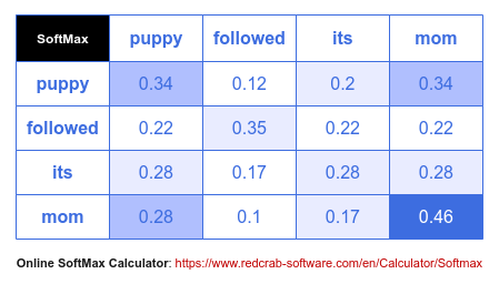
The end result after the third step above, is the normalized and scaled Attention Scores.
The final computation is the dot product of the matrix $V$ (represents all the words of the sentence) with the just determined Attention Scores. The effect of this operation is like finding the weighted sum of all the words with respect to the other words in the matrix $V$. In essense, it is making the words of the sentence CONTEXT AWARE using some kind of weights aka the Attention Scores.
In effect, the Attention mechanism is AMPLIFYING words that are related and FILTERING out words that add no value.
The observant readers may be thinking - there are no parameters (or Weights) in the Attention block of Figure.6 above that could be adjusted during the model training ???
What we illustrated in the Figure.6 above was for simplicity and better understanding. In order to make the Attention block learn during the model training, we introduce linear neural network layers to the Attention block of Figure.6 above, which results in the following illustration:
Hope this clarifies the crux of the idea behind the concept of Self-Attention mechanism !!!
Moving along, the next part of the paper to unravel is the Multi-Head Attention from the block in Figure.5 above.
To determine the Attention Scores, we started with the embedding vectors of the words in the sentence and fed them to the Attention block of Figure.12 above. What if we fed the embedding vectors of the words in the sentence to many instances of the Attention block of Figure.12 above, with the thought that each of the instances will learn quite different patterns ???
The following illustration depicts three instances of the Attention block of Figure.12 above, each processing the word embedding vectors, with the belief that they will each learn different set of patterns:
The Attention Scores from the three instances can then be combined and fed into a linear neural network layer to produce the final Attention Scores. The idea is that the linear neural network will learn from multiple perspectives to produce more refined final scores.
The final puzzle piece from the Transformer model in Figure.2 above is the Positional Encoding.
In the Seq2Seq model, the input tokens (words) from a sentence are processed in sequential order and hence did not have the need to indicate the position of the words. However, in the Transformer model, the input tokens (words) from a sentence are processed in parallel. This poses an interesting challenge.
To understand the situation, consider the following two sentences:
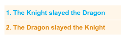
To two sentences indicated above have identical words, except that they have totally different meaning.
In order to ensure the position of the words in a sentence are preserved during parallel processing, it somehow needs to be encoded into the word embedding vectors.
One naive approach could be to use the index position of each word, converting it to a vector and adding it to the word embedding vector.
The following illustration shows this naive approach:
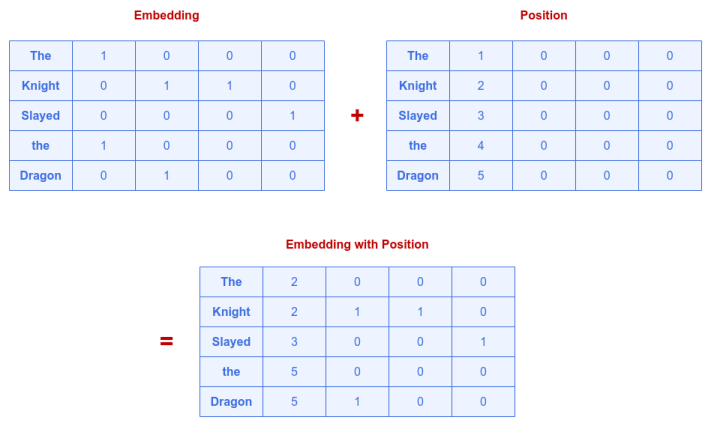
This naive approach completely distorts the embedding vector and may break the similarity between words. In fact, look at the embedding for the word the in the above illustration - it has been completely changed.
Clearly, this naive approach will NOT work !!!
We need a way to keep the position values bounded, such that, they do not significantly change the word embedding, but at the same time have infinite values (to support very long sentences). This is why the researcher of the paper chose to use the sine and cosine functions. These functions are bounded in the range $[-1, 1]$ and extend to infinite position.
One challenge with these two Trigonometric functions - they repeat at regular frequencies. To fix the issue, two things can be done - first change the frequency to a lower value and second alternate between the two Trigonometric functions.
In mathematical terms, the sine function can be written as follows:
$y = a.sin(b.x)$
and
$y = a.cos(b.x)$
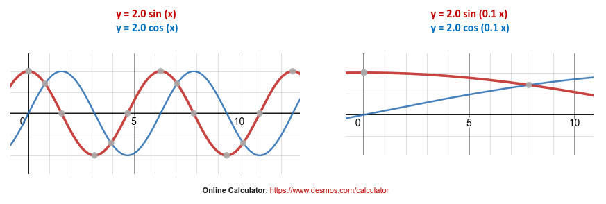
where the variable $a$ controls the height (or amplitude) and the variable $b$ controls the horizontal stretch (or frequency). The lower the value of $b$, the farther it is stretched.
The following graphs illustrate the effect of variable $a$ and $b$:
To ensure the encoded values do not repeat the variable $b$ is set as $\Large{\frac{pos}{10000^{2i/d}}}$
where:
$pos$ is the position of the word starting at $1$ for the first word, $2$ for the second and so on
$i$ is the array index of the element within the embedding vector. If the embedding vector is of size $4$, then it has $4$ array elements and the index $i$ ranges from $0$ to $3$
$d$ is the size of the embedding vector
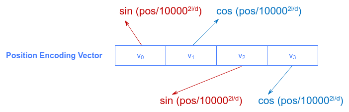
The Positional Encoding vector for each word will have the same size as the word embedding vector with the even array index positions encoded using the sine function and the odd array index positions encoded using the cosine function.
In mathematical terms:
For even array index positions: $sin(\Large{\frac{pos}{10000^{2i/d}}}\normalsize{)}$
For odd array index positions: $cos(\Large{\frac{pos}{10000^{2i/d}}}\normalsize{)}$
The following illustration shows how the array elements of the Positional Encoding vector are encoded:
With this, we have all the blocks from Figure.2 unpacked and revealed.
References