Deep Learning - Word Embeddings with Word2Vec

Bhaskar S

09/04/2023

Introduction

Great progress has been made in the field of Natural Language Processing (or NLP for short) due to the various advances in Deep Learning. Modern NLP models can be trained using vast amounts of textual content and they in turn are able to generate new text content, translate text from one langauge to another, engage in a conversational dialog, and a lot more.

At the heart of all the Deep Learning models lies the complex mathematical machinery which takes in numbers, processes them via the mathematical machinery, and in the end spits out numbers. So, how are the vast amounts of text data consumed by the Deep Learning models ???

This is where the concept of Word Embeddings comes into play, which enables one to map words from the text corpus (referred to as the vocabulary) into corresponding numerical vectors in an n-dimensional space. One of the benefits of representing the words as vectors in an n-dimensional space for the given text corpus is that the surrounding $N$ words to the left or right (known as the context window) of any word from the corpus tend to appear close to one another in the n-dimensional space.

Word to Vector (or Word2Vec for short) is an approach for creating Word Embeddings from any given text corpus.

There are two Word2Vec techniques for creating Word Embeddings which are as follows:

Skip Gram
Continuous Bag of Words (or CBOW for short)

Word2Vec in Detail

For the rest of the sections in this article, let us consider the following three senetences to be the text corpus:

[
  'Alice drinks a glass of water after her exercise',
  'Bob likes to drink orange juice in the morning',
  'Charlie enjoys a cup of Expresso for breakfast'
]

The vocabulary from the text corpus after taking out all the stop words will be following set of unique words:

[
  'alice', 'drinks', 'glass', 'water', 'exercise', 'bob', 'likes', 'drink', 'orange', 'juice', 'morning', 'charlie', 'enjoys', 'cup',
  'expresso', 'breakfast'
]

Given that any Deep Neural Network model only works with numbers, how do we translate the words in the vocabulary to numbers ???

In order to translate words to numbers, we use the technique of One-Hot Encoding. We assign a unique index position to each of the words in our vocabulary as shown below:

{
  'breakfast': 0,
  'expresso': 1,
  'cup': 2,
  'enjoys': 3,
  'charlie': 4,
  'morning': 5,
  'juice': 6,
  'orange': 7,
  'drink': 8,
  'likes': 9,
  'bob': 10,
  'exercise': 11,
  'water': 12,
  'glass': 13,
  'drinks': 14,
  'alice': 15
}

To create a One-Hot Encoded vector for any word, we create a vector of size 16, with a '1' in the index position corresponding to the word, and '0' in the other positions.

For example, the One-Hot Encoded vector for the word 'morning' would be as follows:

[0, 0, 0, 0, 0, 1, 0, 0, 0, 0, 0, 0, 0, 0, 0, 0]

Similarly, the One-Hot Encoded vector for the word 'expresso' would be as follows:

[0, 1, 0, 0, 0, 0, 0, 0, 0, 0, 0, 0, 0, 0, 0, 0]

At this point, a question may arise in ones mind - we just encoded words from the corpus to corresponding numerical vectors using the simple One-Hot Encoding approach. Is this not good enough ???

Well, one of the challenges with a One-Hot Encoded vector is that it DOES NOT capture any context of the word. In other words, there is no information about the possible surrounding words or similarities from the corpus captured.

The next question that may pop in ones mind - what does it mean for two numerical vectors to be close to each other in the n-dimensional space.

To get an intuition on this, let us consider two numerical vectors in a 2-dimensional coordinate space, which is easier to visualize.

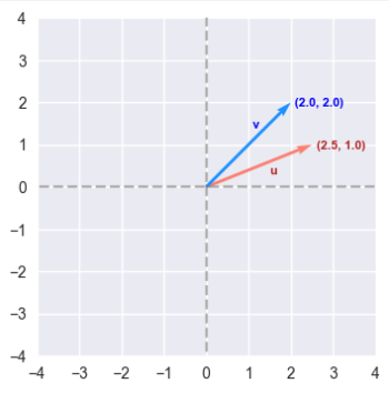
The following illustration depicts two numerical vectors $u$ and $v$ (of size $2$) in a 2-dimensional coordinate space:

Figure.1

The dot product $u.v^T$ of the vectors $u$ and $v$ indicates the strength of the closeness or similarity between the two vectors.

$u.v^T = \begin{bmatrix} 2.5 & 1.0 \end{bmatrix} * \begin{bmatrix} 2.0 \\ 2.0 \end{bmatrix} = 2.5* 2.0 + 1.0*2.0 = 5.0 + 2.0 = 7.0$ $..... \color{red}\textbf{(1)}$

The following illustration depicts two numerical vectors $u$ and $w$ (of size $2$) in a 2-dimensional coordinate space:

Figure.2

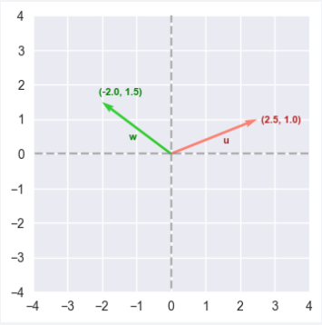
The dot product $u.w^T$ of the vectors $u$ and $w$ can be computed as follows:

$u.w^T = \begin{bmatrix} 2.5 & 1.0 \end{bmatrix} * \begin{bmatrix} -2.0 \\ 1.5 \end{bmatrix} = 2.5* (-2.0) + 1.0*1.5 = -5.0 + 1.5 = -3.5$ $..... \color{red}\textbf{(2)}$

Comparing equations $\color{red}\textbf{(1)}$ and $\color{red}\textbf{(2)}$, we notice that the value of equation $\color {red}\textbf{(1)}$ is greater than the value of $\color{red}\textbf{(2)}$. Hence the vectors $u$ and $v$ are closer, which is obvious by visually looking at Figure.1 above.

This same argument can be extended to vectors in the n-dimensional space.

Skip Gram

In the following sections, we will explain the Skip Gram model for Word Embedding.

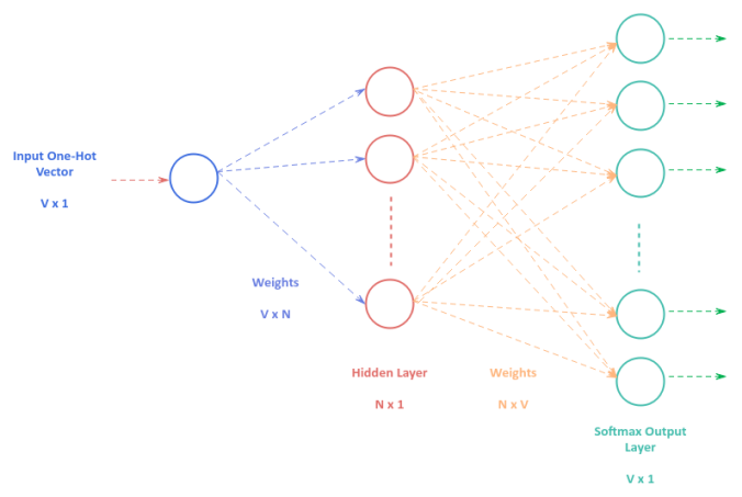
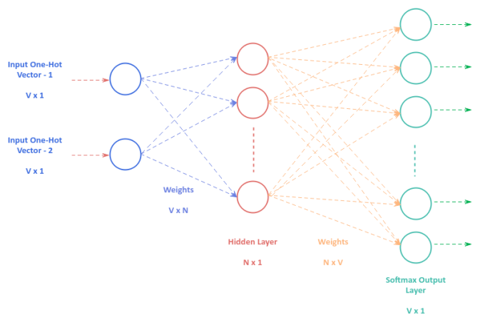
The following illustration depicts the Neural Network model with one hidden layer that is used by the Skip Gram technique:

Figure.3

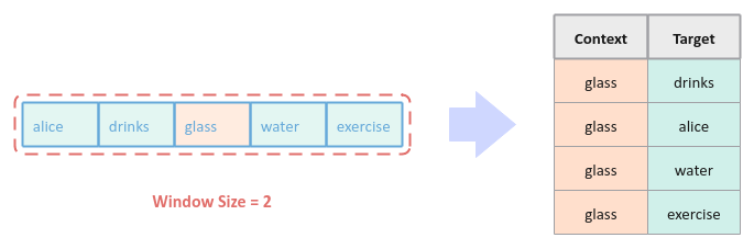
We need to create a data set for training the Neural Network model for Skip Gram. Assuming we choose a window size of $2$, for every sentence in the corpus, we pick a word at random, referred to as the context word, and then find the surrounding left and right words of the window size from the context word.

The following illustration depicts the scenario of picking the word 'glass' at random from the first sentence of our text corpus and the identifying the surrounding words to generate the corresponding training data (table on right):

Figure.4

Similarly, the following illustration depicts the scenario of picking the word 'orange' at random from the second sentence of our text corpus and the identifying the surrounding words to generate the corresponding training data (table on right):

Figure.5

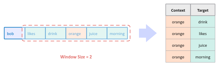
In essence, with the Skip Gram technique, we are trying to predict the surrounding words given a context word.

To train the Neural Network model for Skip Gram, we feed the training data of the One-Hot Encoded context word vectors to the input layer (of size $V$), which passes through a single hidden layer consisting of $N$ neurons, before finally producing outcomes from the output layer via the softmax activation function (of size $V$). If the the predicted outcome is not the surrounding target words, we adjust the weights of the Neural Network through backpropagation.

Once the Neural Network model for Skip Gram is trained well enough, the weights from the hidden layer to the output layer capture the word embeddings for the text corpus.

Continuous Bag of Words

In the following sections, we will explain the Continuous Bag of Words model (CBOW for short) for Word Embedding.

The following illustration depicts the Neural Network model with one hidden layer that is used by the CBOW technique:

Figure.6

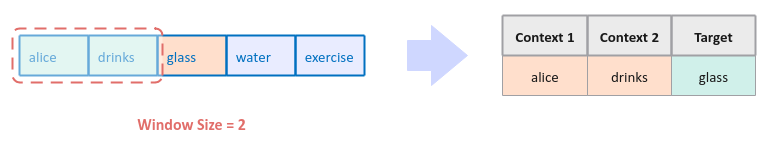
We need to create a data set for training the Neural Network model for CBOW . Assuming we choose a window size of $2$, for every sentence in the corpus, we pick a word at random, referred to as the target word, and then find the surrounding left words (referred to as the context words) of the window size from the target word.

The following illustration depicts the scenario of picking the word 'glass' at random from the first sentence of our text corpus and the identifying the surrounding context words to generate the corresponding training data (table on right):

Figure.7

Next, we select the word to the right of the target word to be the new target word and then find the surrounding context words to the left of the target word to generate the corresponding training data (table on right):

Figure.8

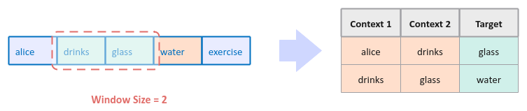
We continue this process until we reach the last word as the target word in the first sentence.

Next, we pick a random from the next sentence and so on to continue the process till we have identified all the sets from the text corpus.

In essence, with the CBOW technique, we are trying to predict the target word given the context words.

The training of the Neural Network model for CBOW is similar to that of Skip Gram, except that the input layer takes multiple context words as input as depicted in Figure.6 above.

Hands-on Word2Vec Using Gensim

For the hands-on demonstration of Word Embeddings, we will make use of the popular Python library called Gensim.

The installation and setup of Gensim will be performed on a Ubuntu 22.04 LTS Linux desktop with the Python 3 programming language installed.

Open a Terminal window to perform the necessary installation step(s).

To install Gensim, execute the following command:

$ sudo pip3 install gensim

This above command will install all the required dependencies along with the desired Gensim package.

All the code snippets will be executed in a Jupyter Notebook code cell.

To import the necessary Python module, execute the following code snippet:

import nltk
from gensim.models import Word2Vec
from nltk.corpus import stopwords
from nltk.tokenize import WordPunctTokenizer

Assuming the logged in user is alice, to set the correct path to the nltk data packages, execute the following code snippet:

nltk.data.path.append("/home/alice/nltk_data")

To create an instance of the stop words and the word tokenizer, execute the following code snippet:

stop_words = stopwords.words('english')
word_tokenizer = WordPunctTokenizer()

To cleanse the sentences from our text corpus by removing the punctuations, stop words, two-letter words, etc., execute the following code snippet:

cleansed_corpus_tokens = []
for txt in text_corpus:
  tokens = word_tokenizer.tokenize(txt)
  final_words = [word.lower() for word in tokens if word.isalpha() and len(word) > 2 and word not in stop_words]
  cleansed_corpus_tokens.append(final_words)
cleansed_corpus_tokens[:5]

The following would be a typical output:

Output.1

[['alice', 'drinks', 'glass', 'water', 'exercise'],
 ['bob', 'likes', 'drink', 'orange', 'juice', 'morning'],
 ['charlie', 'enjoys', 'cup', 'expresso', 'breakfast']]

The gensim module implements both the Word2Vec models.

To create an instance of the Skip Gram model, execute the following code snippet:

word2vec_model = Word2Vec(sg=1, alpha=0.05, window=3, min_count=0, workers=2)

When the parameter sg=1, the Skip Gram model is used. The parameter min_count=0 indicates that the model ignore words with total frequency lower that the specified value. The parameter workers=2 indicates the number of threads to use for faster training.

To build the vocabulary for the text corpus, execute the following code snippet:

word2vec_model.build_vocab(cleansed_corpus_tokens)

To train the Word2Vec model for Skip Gram, execute the following code snippet:

word2vec_model.train(cleansed_corpus_tokens, total_examples=word2vec_model.corpus_count, epochs=2500)

The parameter total_examples=word2vec_model.corpus_count indicates the count of sentences in the text corpus.

Given the text corpus is very small, we need to train the model for a number of iterations, which is controlled by the parameter epochs=2500.

Once the Word2Vec model is trained, the Word Embeddings are stored in the object word2vec_model.wv.

To save the trained model to disk at location '/home/alice/models', execute the following code snippet:

model_loc = '/home/alice/models/w2v-sg.model'
word2vec_model.save(model_loc)

To load the previously saved model from disk at location '/home/alice/models', execute the following code snippet:

w2v_model = Word2Vec.load(model_loc)

To retrieve and display the top three words in the vicinity of the word 'juice', execute the following code snippet:

w2v_model.wv.most_similar('juice', topn=3)

The following would be a typical output:

Output.2

[('bob', 0.9977365732192993),
 ('drink', 0.9975760579109192),
 ('orange', 0.997246265411377)]

Notice the model has predicted with great accuracy the surrounding words for the given word 'juice'.

References

Gensim Documentation

Original Google Paper on Word2Vec

Introduction to Deep Learning - Part 3

Introduction to Deep Learning - Part 2

Introduction to Deep Learning - Part 1