Figure.1
| PolarSPARC |
Document Similarity using NLTK and Scikit-Learn
| Bhaskar S | 02/17/2023 |
Overview
In the articles, Basics of Natural Language Processing using NLTK and Feature Extraction for Natural Language Processing, we covered the necessary ingredients of Natural Language Processing (or NLP for short).
Document Similarity in NLP determines how similar documents (textual data) are to each other using their vector representation.
In this following sections, we will demonstrate how one can determine if two documents (sentences) are similar to one another using nltk and scikit-learn.
Mathematical Intuition
In order to perform any type of analysis, one needs to convert a text document into a feature vector, which was covered in the article Feature Extraction for Natural Language Processing.
Once we have a vector representation of a text document, how do we measure the similarity between two documents ???
This is where Linear Algebra comes into play.
To get a better understanding, let us start with a very simple example. Assume a corpus that has four documents, each with only two unique words describing them. This implies the vector representation of each document will have only two elements, which can easily be represented in a two-dimensional coordinate space.
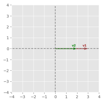
The following would be the graph for two documents (represented as vectors) that contain similar count of the same words:
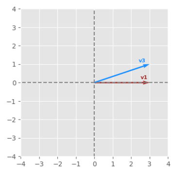
The following would be the graph for two documents (represented as vectors) that contain one word in common and the other different:
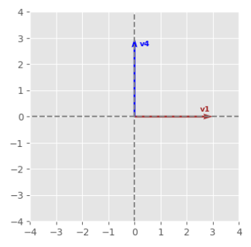
The following would be the graph for two documents (represented as vectors) that contain totally different words:
From the illustrations above, we can infer that the Document Similarity is related to the angle between the two vectors. This measure is referred to as the Cosine Similarity. The smaller the angle, the closer the documents in similarity.
From Linear Algebra, we know that the dot product of two vectors $\vec{a}$ and $\vec{b}$ in a two dimensional space is the cosine of the angle between the two vectors multiplied with the lengths of the two vectors.
In other words:
$a^Tb = \sum\limits_{i=1}^n\vec{a_i}\vec{b_i} = \lVert \vec{a} \rVert \lVert \vec{b} \rVert \cos \theta$
Note that $\theta$ is the angle between the two vectors $\vec{a}$ and $\vec{b}$.
Rearranging the equation, we get:
$\cos \theta = \Large{\frac{a^Tb}{\lVert \vec{a} \rVert \lVert \vec{b} \rVert}}$
The following graph is the illustration of the two vectors:
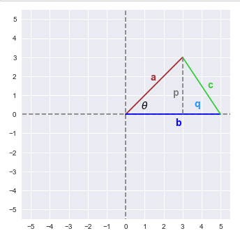
From the triangle above, using the Pythagorean Theorem, we can infer the following:
$c^2 = p^2 + q^2$ ..... $\color{red} (1)$
$a^2 = p^2 + (b-q)^2$ ..... $\color{red} (2)$
Using Trigonometry, we can infer the following:
$\sin \theta = \Large{\frac{p}{a}}$ OR $p = a \sin \theta$ ..... $\color{red} (3)$
$\cos \theta = \Large{\frac{b-q}{a}}$ OR $q = b - a \cos \theta$ ..... $\color{red} (4)$
Expanding the equation $\color{red} (2)$ from above, we get:
$p^2 + (b^2 + q^2 - 2bq) = a^2$
That is:
$(p^2 + q^2) + b^2 -2bq = a^2$
Replacing the first term with $c^2$ from equation $\color{red} (1)$ above, we get:
$c^2 + b^2 -2bq = a^2$
Replacing q from equation $\color{red} (4)$ above, we get:
$c^2 + b^2 -2b(b - a \cos \theta) = a^2$
Simplifying, we get:
$c^2 = a^2 + b^2 - 2ab \cos \theta = {\lVert \vec{a} \rVert}^2 + {\lVert \vec{b} \rVert}^2 - 2\lVert \vec{a} \rVert \lVert \vec{b} \rVert \cos \theta$
From geometry, we can infer $\vec{c} = \vec{a} - \vec{b}$
In other words:
$\lVert \vec{c} \rVert = \lVert \vec{a} \rVert - \lVert \vec{b} \rVert$
We know $\lVert \vec{a} \rVert = a^Ta$. Therefore, rewriting the above equation as:
$\lVert \vec{c} \rVert = (a - b)^T(a - b) = a^Ta - 2a^Tb + b^Tb = {\lVert \vec{a} \rVert}^2 + {\lVert \vec{b} \rVert}^2 - 2a^Tb$
Substituting in the equation for the law of cosines, we get:
${\lVert \vec{a} \rVert}^2 + {\lVert \vec{b} \rVert}^2 - 2a^Tb = {\lVert \vec{a} \rVert}^2 + {\lVert \vec{b} \rVert}^2 - 2ab \cos \theta$
Simplifying the equation, we get:
$a^Tb = \lVert \vec{a} \rVert \lVert \vec{b} \rVert \cos \theta$
Thus proving the geometric interpretation of the vector dot product.
This concepts applies to two vectors in the n-dimensional hyperspace as well.
Installation and Setup
Please refer to the article Feature Extraction for Natural Language Processing for the environment installation and setup.
Open a Terminal window in which we will excute the various commands.
To launch the Jupyter Notebook, execute the following command in the Terminal:
$ jupyter notebook
Hands-On Document Similarity
The first step is to import all the necessary Python modules such as, pandas, nltk, matplotlib, scikit-learn, and wordcloud by running the following statements in the Jupyter cell:
import nltk
import numpy as np
import pandas as pd
import matplotlib.pyplot as plt
from collections import defaultdict
from nltk.corpus import stopwords
from nltk.tokenize import WordPunctTokenizer
from sklearn.feature_extraction.text import TfidfVectorizer
from sklearn.metrics.pairwise import cosine_similarity
from wordcloud import WordCloud
To set the correct path to the nltk data packages, run the following statement in the Jupyter cell:
nltk.data.path.append("/home/alice/nltk_data")
To initialize the tiny corpus containing 4 sentences for ease of understanding, run the following statement in the Jupyter cell:
documents = [
  'Python is a high-level, general-purpose programming language that is dynamically typed and garbage-collected.',
  'Go is a statically typed, compiled high-level programming language designed with memory safety, garbage collection, and CSP-style concurrency.',
  'Java is a high-level, class-based, object-oriented programming language that is designed to have as few implementation dependencies as possible.',
  'Leadership encompasses the ability of an individual, group or organization to "lead", influence or guide other individuals, teams, or entire organizations.'
]
To load the Stop Words from the English language defined in nltk, run the following statement in the Jupyter cell:
stop_words = stopwords.words('english')
To initialize an instance of a word tokenizer, run the following statement in the Jupyter cell:
word_tokenizer = WordPunctTokenizer()
To initialize an instance of the wordnet lemmatizer, run the following statement in the Jupyter cell:
word_lemmatizer = nltk.WordNetLemmatizer()
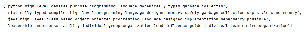
To cleanse the sentences from the corpus by removing the punctuations, two-letter words, converting words to their roots, collecting all the unique words from the corpus, and display the cleansed sentences, run the following statements in the Jupyter cell:
vocabulary_dict = defaultdict(int)
cleansed_documents = []
for doc in documents:
    tokens = word_tokenizer.tokenize(doc)
    alpha_words = [word.lower() for word in tokens if word.isalpha() and len(word) > 2 and word not in stop_words]
    final_words = [word_lemmatizer.lemmatize(word) for word in alpha_words]
    for word in final_words:
        vocabulary_dict[word] += 1
    cleansed_doc = ' '.join(final_words)
    cleansed_documents.append(cleansed_doc)
cleansed_documents
The following would be a typical output:
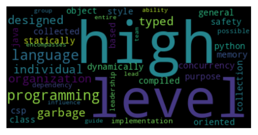
To display a word cloud of all the unique words (features) from the corpus, run the following statements in the Jupyter cell:
word_cloud = WordCloud()
word_cloud.generate_from_frequencies(vocabulary_dict)
plt.imshow(word_cloud, interpolation='bilinear')
plt.axis('off')
plt.show()
The following would be a typical output:
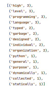
To display the first 15 most frequently occuring unique words from our corpus, run the following statements in the Jupyter cell:
sorted_vocabulary = sorted(vocabulary_dict.items(), key=lambda kv: kv[1], reverse=True)
sorted_vocabulary[:15]
The following would be a typical output:
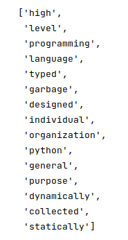
To collect all the unique words from the corpus into a list and display the first 15 vocabulary entries, run the following statements in the Jupyter cell:
vocabulary = []
for word, count in sorted_vocabulary:
    vocabulary.append(word)
vocabulary[:15]
The following would be a typical output:
To create an instance of the TF-IDF vectorizer, run the following statement in the Jupyter cell:
word_vectorizer = TfidfVectorizer(vocabulary=vocabulary)
To create a new TF-IDF scores vector for our corpus, run the following statement in the Jupyter cell:
matrix = word_vectorizer.fit_transform(cleansed_documents).toarray()
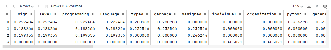
To create a pandas dataframe for the TF-IDF scores vector and display the rows of the dataframe, run the following statements in the Jupyter cell:
documents_df = pd.DataFrame(data=matrix, columns=vocabulary)
documents_df
The following would be a typical output:
To compute and display the cosine similarity score between the first document compared to the other documents in the corpus, run the following statements in the Jupyter cell:
first_doc = matrix[0].reshape(1, -1)
for i in range(1, len(matrix)):
    next_doc = matrix[i].reshape(1, -1)
    similarity_score = cosine_similarity(first_doc, next_doc)
    print(f'Doc-1 vs Doc-{i+1} => {similarity_score}')
The following would be a typical output:
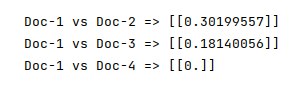
As is evident from the Figure.10 above, the first and the second document are more similar than the others in the corpus, which makes sense as they are related to the topic of high-level programming languages with garbage collection. The fourth document is related to leadership and hence not similar.
Jupyter Notebook
The following is the link to the Jupyter Notebook that provides an hands-on demo for this article:
References