Figure.1
| PolarSPARC |
Machine Learning - Polynomial Regression using Scikit-Learn - Part 3
| Bhaskar S | 03/27/2022 |
Overview
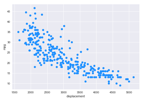
In Part 2 of this series, we demonstrated the Linear Regression models using Scikit-Learn. For the Simple Linear Regression of Displacement vs MPG, our model achieved an $R^2$ score of about $65\%$, which is not that great. Also, observe the scatter plot that depicts the relationship between displacement and mpg from the auto mpg test dataset as shown below:
Notice that the relationship follows a NON-LINEAR (curved) path from top-left to the bottom-right.
Basics of Polynomials
The word Polynomial is in fact a composition of two terms - Poly which means MANY, and Nomial which means TERMS. In Algebra, a polynomial is function that consists of constants, coefficients, variables, and exponents.
For any polynomial equation, the variable with the largest exponent determines the Degree of the polynomial. For example, $y = x^3 - 4x + 5$ is a third degree (cubic) polynomial equation, which has the constant $5$, the variable $x$ with coefficient $4$ and an exponent $x^3$ with coefficient $1$. This is a third-degree polynomial or also known as a Cubic polynomial.
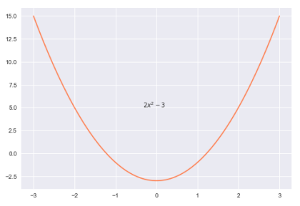
To get an intuition on the shapes of the various polynomial equations, let us look at some of the polynomial plots.
The following plot illustrates a 2nd-degree polynomial equation:
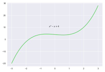
The following plot illustrates a 3nd-degree polynomial equation:
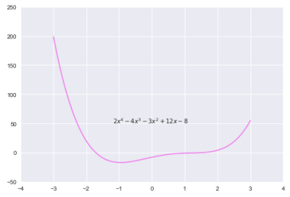
The following plot illustrates a 4th-degree polynomial equation:
Polynomial Regression
The purpose of the Polynomial Regression is to find a polynomial equation of the form $y = \beta_0 + \beta_1.x + \beta_2.x^2 + ... + \beta_n.x^n$ (of degree $n$) such that, it estimates the non-linear relationship between the dependent outcome (or target) variable $y$ and one or more independent feature (or predictor) variables $x_1, x_2, ..., x_n$.
In other words, one can think of the Polynomial Regression as an extension of the Linear Regression, with the difference that it includes polynomial terms to deal with the non-linear relationship.
Assuming $m$ dependent output values and a $n$ degree polynomial, the following is the matrix representation:
$\begin{bmatrix} y_1 \\ y_2 \\ ... \\ y_m \end{bmatrix} = \begin{bmatrix} 1 & x_1 & x_1^2 & ... & x_1^n \\ 1 & x_2 & x_2^2 & ... & x_2^n \\ ... & ... & ... & ... & ... \\ 1 & x_m & x_m^2 & ... & x_m^n \end{bmatrix} \begin{bmatrix} \beta_0 \\ \beta_1 \\ ... \\ \beta_n \end{bmatrix}$
Using the matrix notation, we arrive at $\hat{y} = X\beta$, where $X$ is a matrix. Notice that this form of mathematical representation is very similar to that of the Multiple Linear Regression.
The mathematical derivation follows the same set of steps as was the case with the Multiple Linear Regression we explored in Part 1 of this series, so we will skip it here.
For the demonstration of the polynomial regression, we will cover the model that estimates mpg using displacement.
The first step is to import all the necessary Python modules such as, matplotlib, pandas, and scikit-learn as shown below:
import pandas as pd
import matplotlib.pyplot as plt
from sklearn.model_selection import train_test_split
from sklearn.preprocessing import PolynomialFeatures
from sklearn.linear_model import LinearRegression
from sklearn.metrics import r2_score
The next step is to load the auto mpg dataset into a pandas dataframe and assign the column names as shown below:
url = 'https://archive.ics.uci.edu/ml/machine-learning-databases/auto-mpg/auto-mpg.data'
auto_df = pd.read_csv(url, delim_whitespace=True)
auto_df.columns = ['mpg', 'cylinders', 'displacement', 'horsepower', 'weight', 'acceleration', 'model_year', 'origin', 'car_name']
The next set of steps, related to exploratory data analysis, help cleanse and prepare the data for regression. We will skip those, since we covered them in detail in Part 2 of this series.
The next step is to create the training dataset and a test dataset with the desired feature (or predictor) variable. We create a 75% training dataset and a 25% test dataset with the feature variable displacement as shown below:
X_train, X_test, y_train, y_test = train_test_split(auto_df[['displacement']], auto_df['mpg'], test_size=0.25, random_state=101)
The next step is to initialize the polynomial feature class from scikit-learn. Think of the polynomial feature object as a feature transformer that takes one-dimensional features to generate features of the higher dimension based on the specified degree of the polynomial. For our demonstration, we will initialize a quadratic polynomial feature transformer (degree=2) with the line-intercept (include_bias=True) as shown below:
transformer = PolynomialFeatures(degree=2, include_bias=True)
The next step is to transform the training dataset to include $2^{nd}$ degree features as shown below:
X_p_train = transformer.fit_transform(X_train)
The next step is to initialize the linear regression model class as shown below:
model = LinearRegression()
The next step is to train the model using the training dataset as shown below:
model.fit(X_train, y_train)
The next step is to display the values for the intercept and the polynomial coefficients as shown below:
model.intercept_, model.coef_
The following illustration displays the values for the intercept and the polynomial coefficient from the model:
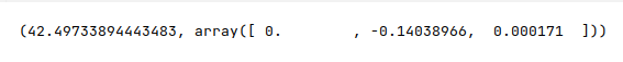
Notice that the coefficients for the other polynomial terms are included in the output above.
The next step is to transform the test dataset to include $2^{nd}$ degree features as shown below:
X_p_test = transformer.fit_transform(X_test)
The next step is to use the trained model to predict the mpg using the test dataset as shown below:
y_predict = model.predict(X_p_test)
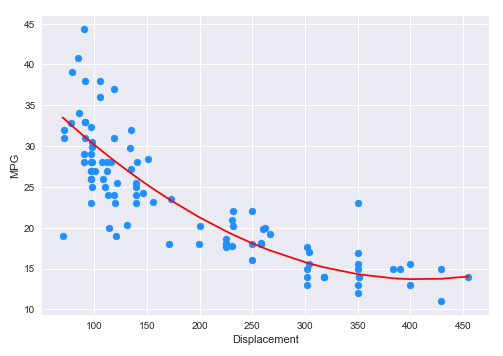
The next step is to display a scatter plot (along with the polynomial curve of best fit) that shows the visual relationship between the data from the columns displacement and mpg from the auto mpg test dataset as shown below:
plt.scatter(X_test, y_test, color='dodgerblue')
sorted_Xy = sorted(zip(X_test.displacement, y_predict))
X_s, y_s = zip(*sorted_Xy)
plt.plot(X_s, y_s, color='red')
plt.xlabel('Displacement')
plt.ylabel('MPG')
plt.show()
The following illustration shows the scatter plot (along with the polynomial curve of best fit) between displacement and mpg from the auto mpg test dataset:
The final step is to display the $R^2$ value for the model as shown below:
r2_score(y_test, y_predict)
The following illustration displays the $R^2$ value for the model:
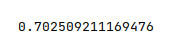
Notice our model has achieved an $R^2$ score of about $70\%$ which is a little better.
Overfitting
One of the challenges with the polynomial regression, especially with the higher degree polynomials, is that the model tends to learn and fit every data point from the training set, including outliers. In other words, the regression model starts to include noise into model, rather than generalizing the genuine underlying relationship between the dependent and independent variables. This behavior of the polynomial regression model is known as Overfitting.
The result of overfitting is as though the regression model was custom made for the given training dataset, which reduces the models ability to be generalized for future predictions.
Hands-on Demo
The following is the link to the Jupyter Notebook that provides an hands-on demo for this article:
References