First 5
| PolarSPARC |
Introduction to Statistics - Part 3
| Bhaskar S | 07/18/2021 |
In Part 2 of the series, we introduced the concepts around the various probability distributions, namely, the Binomial, the Poisson, and the Normal probability distributions.
In this part of the series, we will delve into the world of Inferential Statistics that focuses on analyzing the data about the sample to arrive at a conclusion about the population. In particular, we will look at the Central Limit Theorem, the Point Estimation, and the Confidence Interval.
Basic Definitions - I
A Sampling Distribution is the probability distribution of a sample statistic (such as the mean, variance, etc) that is formed when samples of size n are repeatedly taken from a population.
Each of the measurements, such as the mean, the standard deviation, etc., from the population is referred to as a Parameter.
Each of the measurements, such as the mean, the standard deviation, etc., from the sample is referred to as a Statistic.
Central Limit Theorem
The Central Limit Theorem is one of the core foundations for inferential statistics as it provides information about the sample mean \(\bar{x}\) to make inferences about the population. It states the following:
For any population that is NOT normally distributed, the sampling distribution of the sample means \(\bar{x}\) will approximate a normal distribution provided the sample size n is large
For a normally distributed population, the sampling distribution of sample means is normally distributed for any sample size n
The sample mean \(\mu_{\bar{x}}\) = the population mean \(\mu\). That is, \(\mu_{\bar{x}}\) = \(\mu\)
The sample standard deviation \(\sigma_{\bar{x}}\) = the population standard deviation \(\sigma\) divided by the square root of sample size \(\sqrt{n}\). That is, \(\sigma_{\bar{x}}\) = \(\Large{\frac{\sigma}{\sqrt{n}}}\)
The sample standard deviation \(\sigma_{\bar{x}}\) is also referred to as the Standard Error
To get a better intuition and understanding of the Central Limit Theorem, we will perform some experiments using one years' worth of market close stock data for the symbol UNP.
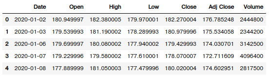
The following illustration shows the first five entries of market close data for the symbol UNP:
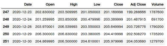
The following illustration shows the last five entries of market close data for the symbol UNP:
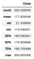
The following illustration shows the summary statistic on the Close price for the symbol UNP:
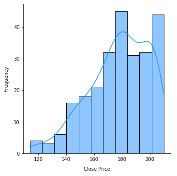
The following illustration shows the distribution of the Close price for the symbol UNP, which is not normally distributed:
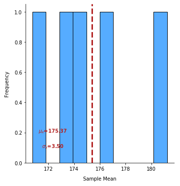
The following illustration shows the sampling distribution for 10 sets of samples of size 5 on the Close price for the symbol UNP:
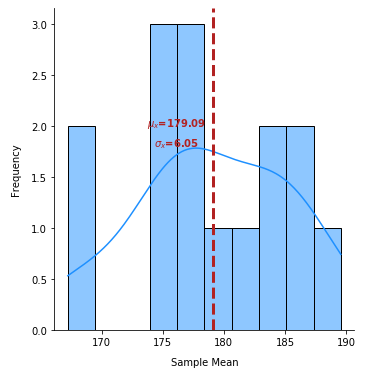
The following illustration shows the sampling distribution for 10 sets of samples of size 15 on the Close price for the symbol UNP:
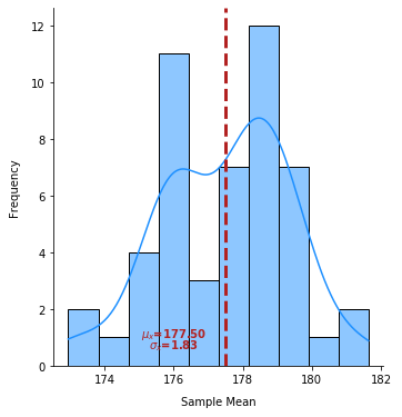
The following illustration shows the sampling distribution for 100 sets of samples of size 50 on the Close price for the symbol UNP:
The following illustration shows the sampling distribution for 100 sets of samples of size 100 on the Close price for the symbol UNP:
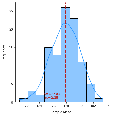
As is evident from the illustration above, as the sample size increases, the sample distribution becomes normally distributed, the mean of the sample distribution approaches the population distribution \(\approx{177.8}\), and the standard deviation of the sample distribution approaches \(\Large{\frac{21.339}{\sqrt{100}}}\), which \(\approx{2.1}\).
In Part 2, we learnt how one could find the probability of a normally distributed random variable x will lie in an interval by calculating the area under the normal curve using the Z-score. Similarly, we can find the probability that a sample mean \(\bar{x}\) will lie in a given interval of the sampling distribution using the Z-score formula: \(\Large{\frac{{\bar{x} - \mu}}{\sigma/\sqrt{n}}}\).
| Example-1 | A study of a fishing lake where the length of a trout taken at random from the pond has a normal distribution with mean \(\mu\) of 10.2 inches and standard deviation \(\sigma\) of 1.4 inches. What is the probability that the mean length \(\bar{x}\) of 5 trouts taken at random is between 8 and 12 inches. |
|---|---|
|
From the Central Limit Theorem, we know \(\mu_{\bar{x}}\) = \(\mu\). That is, \(\mu_{\bar{x}}\) = 10.2 Also, from the Central Limit Theorem, \(\sigma_{\bar{x}}\) = \(\Large{\frac{\sigma}{\sqrt{n}}}\), where n is the size of the sample. That is, \(\sigma_{\bar{x}}\) = \(\Large{\frac{1.4}{\sqrt{5}}}\) \(\approx{0.63}\) To find the probability the sample mean \(\bar{x}\) lies between the interval of 8 to 12 inches, we use the formula \(\Large{\frac{{\bar{x} - \mu}}{\sigma/\sqrt{n}}}\) \(\approx \Large{\frac{\bar{x} - 10.2}{0.63}}\) (A) The first interval \(\mu_{\bar{x}}\) = 8, so z = \(\Large{\frac{8 - 10.2}{0.63}}\) \(\approx{-3.49}\). The area to the left of z = -3.49 is 0.0002 (B) The second interval \(\mu_{\bar{x}}\) = 12, so z = \(\Large{\frac{12 - 10.2}{0.63}}\) \(\approx{2.86}\). The area to the left of z = 2.86 is 0.9979 To find the area between z = -3.49 and z = 2.86, we need to subtract (A) from (B). That is, 0.9979 - 0.0002 = 0.9977. Therefore, the probability of the sample mean length (using a sample size of 5) to be between 8 and 12 inches is 0.9977. |
|
Basic Definitions - II
A Point Estimate is a single value estimate for a population parameter. The sample mean \(\bar{x}\) is said to be an unbiased point estimate of the population mean \(\mu\) if the sample statistic does not overestimate or underestimate the population parameter. From the Central Limit Theorem above, we learnt the mean \(\bar{x}\) of a set of sample means (of sample size n) equals the population mean \(\mu\). In other words, the sample mean \(\bar{x}\) is an unbiased point estimate of the population mean \(\mu\). As the sample size n increases, the variability of the sample mean \(\bar{x}\) decreases as the standard deviation (or standard error) \(\sigma/\sqrt{n}\) decreases.
Using the sample mean \(\bar{x}\) as the point estimate of the population mean \(\mu\), the Margin of Error denoted by E (also referred to as the Sampling Error) is the magnitude of \(|\bar{x} - \mu|\). In other words, E = \(|\bar{x} - \mu|\).
An Interval Estimate is an interval range that is used to estimate a population parameter. To create an interval estimate, use the point estimate as the center of the interval, then add and subtract a margin of error from the point estimate.
A Confidence Level denoted by c, with any value between 0 and 1 (typically 0.90, 0.95, or 0.99) is the probability that the interval estimate contains the population parameter assuming that the estimation process is repeated a large number of times. A confidence level is sometimes referred to as the Degree of Confidence OR the Confidence Coefficient.
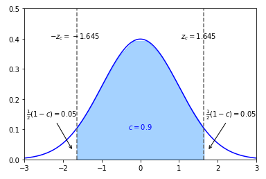
For a confidence level of c, the Critical Value \(z_c\) is the number such that the area under the standard normal curve between \(-z_c\) and \(z_c\) equals c. The critical values are values that separate the sample statistics that are probable from the sample statistics that are improbable or unusual.
The following illustration shows the critical values (\(-z_c\) = -1.645, and \(z_c\) = 1.645) for a confidence level of c = 0.9:
We know the margin of error (also called the Error Tolerance) E = \(|\bar{x} - \mu|\).
We also know the Z-score z = \(\Large{\frac{{\bar{x} - \mu}}{\sigma/\sqrt{n}}}\). Therefore, we can deduce z = \(\Large{ \frac{E}{\sigma/\sqrt{n}}}\). That is, E = \(z\Large{\frac{\sigma}{\sqrt{n}}}\).
For a given confidence level denoted by c and given the population standard deviation \(\sigma\), the margin of error E for the population mean \(\mu\) is E = \(z_c\Large{\frac{\sigma}{\sqrt{n}}}\). This formula is valid only if the sampling distribution satisfies the conditions from the central limit theorem.
Confidence Interval
Now that we know about the point estimate and the margin of error, one can construct an interval estimate for the population parameter \(\mu\). This interval estimate is called the Confidence Interval. In other words, given the confidence level of c, the confidence interval for the population parameter \(\mu\) (when the population parameter \(\sigma\) is known) is: \(\bar{x}-E \lt \mu \lt \bar{x}+E\), where E = \(z_c\Large{\frac{\sigma}{\sqrt{n}}}\).
The main requirements for the sample distribution are similar to the central limit theorem, that is:
For any population that is not normally distributed, the sample size n must be large \(n \ge 30\)
For a normally distributed population, any sample size n is sufficient
The sample mean \(\mu_{\bar{x}}\) = the population mean \(\mu\). That is, \(\mu_{\bar{x}}\) = \(\mu\)
| Example-2 | John jogs 2 miles per day. The standard deviation of his times is 1.80 minutes. During the past year, John has recorded his times to run 2 miles. He has a random sample of 90 of these times. For these 90 times, the mean was 15.60 minutes. Find a 0.95 confidence interval for the mean jogging time for the entire distribution. |
|---|---|
|
Given the sample size n = 90, the mean sample distribution will be normal. Also, given the population standard deviation \(\sigma = 1.80\), we can use the sample mean \(\bar{x} = 15.60\) to find the 95% confidence interval for the population mean \(\mu\). For c = 0.95, the area under the normal curve for the critical value \(\Large{\frac{1}{2}}\)(1 - c) = 0.025. Therefore, the critical value \(z_c\) = 1.96 We know the margin of error E = \(z_c\Large{\frac{\sigma}{\sqrt{n}}}\) = \(1.96\Large{\frac{1.80}{\sqrt{90}}}\) \(\approx 0.37\) We know the confidence interval for the population mean \(\mu\) is \(\bar{x}-E \lt \mu \lt \bar{x}+E\) That is, \(15.60 - 0.37 \lt \mu \lt 15.60 + 0.37\) or \(15.23 \lt \mu \lt 15.97\) Therefore, we can conclude with 95% confidence that the interval is from 15.23 mins to 15.97 mins |
|
For a given sample statistics, as the confidence level c increases, the confidence interval widens. As the confidence interval widens, the precision of the estimate decreases. One way to improve the precision of an estimate without decreasing the confidence level c is to increase the sample size. Given the margin of error E = \(z_c\Large{\frac{\sigma}{\sqrt{n}}}\), we can re-arrange the terms to determine the sample size. In other words, given a confidence level c and a margin of error E, the minimum sample size required to estimate the population mean \(\mu\) is n = \(\Large{(\frac{z_c\sigma}{E})^2}\).
| Example-3 | A research study is designed to find the mean weight of salmon caught by a fishing company. A preliminary study of a random sample of 50 salmon showed a standard deviation of about 2.15 pounds. How large a sample should be taken to be 99% confident that the sample mean is within 0.20 pound of the true mean weight. |
|---|---|
|
For c = 0.99, the area under the normal curve for the critical value \(\Large{\frac{1}{2}}\)(1 - c) = 0.005. Therefore, the critical value \(z_c\) = 2.576 Given the the population standard deviation \(\sigma = 2.15\) and the margin of error E = 0.20. The minimum sample size can be computed using n = \(\Large{(\frac{z_c\sigma}{E})^2}\). That is, n = \(\Large{(\frac{2.576 * 2.15}{0.20})^2}\) = 766.85, which rounds up to 770. |
|
References