Figure.1
| PolarSPARC |
Machine Learning - Data Preparation - Part 3
| Bhaskar S | 05/27/2022 |
Overview
In Part 2 of this series, we used the the City of Ames, Iowa Housing Prices data set to perform the various tasks related to Data Imputation on the loaded data set. In this part, we will first explain the approach to dealing with categorical data that is related to Feature Engineering, followed by hands-on demo in Python.
Feature Engineering - Categorical Data
Categorical feature variables contain string (label) values rather than numerical values. The unique set of the labels is typically a fixed number, where each label represents a specific category.
The following are the two types of categorical feature variables:
Nominal - Consist of a finite set of discrete label values with no specific rank (or order) relationship between those label values. For example, the color of eyes - black, brown, grey, etc., is just that with no one color better (or worse) than the other
Ordinal - Consist of a finite set of discrete label values, which have a specific rank ordering between those label values. For example, the condition of a car - fair, good, excellent, etc
As indicated earlier, all machine learning models require that all the feature variable values be numerical. This implies that all the categorical feature variables be transformed to numerical values.
Data Encoding is the process of replacing all the categorical string values (labels) from the categorical feature variables into numerical values, so that those features can be used by the machine learning models for both training and testing.
The following are some of the commonly used strategies for categorical data encoding:
Ordinal Encoding - Each unique category label is assigned a unique integer value. For example, for the condition of a car, fair is 1, good is 2, excellent is 3, and so on. One thing to keep in mind - it imposes an ordinal relationship and it may be a challenge for some categorical features which have no such ordering. For example, for the eye color, black is 1, brown is 2, grey is 3, and so on
Label Encoding - Used when a categorical target variable needs to be encoded for the classification problems. It is similar to the Ordinal Encoding, except that it expects a single one-dimensional target variable
One-Hot Encoding - Encodes a categorical feature variable into a set of dummy binary feature variables, where each dummy binary variable represents one of the categorical labels. Each dummy binary feature variable will take on a boolean value of either a 0 or a 1, where a 1 represents the presence of the label value and a 0 represents an absence of the label value. For example, if a categorical feature representing the condition of a car takes on the values fair, good, and excellent, then it would be encoded using three dummy binary feature variables called fair, good, and excellent corresponding to each of the three label values. When a sample (row in the dataframe) has the value of good, then the dummy binary variable fair will encoded as 0, the dummy binary variable good will be encoded as 1, and the dummy binary variable excellent will be encoded as 0.
For a categorical feature variable with $k$ label values, one will end up with $k$ additional dummy binary feature variables in the data set. One optimization could be to use $k-1$ dummy binary feature variables to encode the label values of the categorical feature. For example, if a sample (row in the dataframe) has the value of excellent, then the dummy binary variable fair will encoded as 0 and the dummy binary variable good will be encoded as 0. With this, one can implicitly conclude that excellent is a 1
Hands-On Data Encoding
The first step is to import all the necessary Python modules such as, pandas and transformers from scikit-learn as shown below:
import pandas as pd
import matplotlib.pyplot as plt
from sklearn.preprocessing import StandardScaler
The next step is to load and display the imputed housing price dataset into a pandas dataframe as shown below:
url = './data/ames-imputed.csv'
home_price_df = pd.read_csv(url, keep_default_na=False)
home_price_df
Notice the use of the option keep_default_na, which is very important. Else, the string labels 'NA' will be interpreted as nulls.
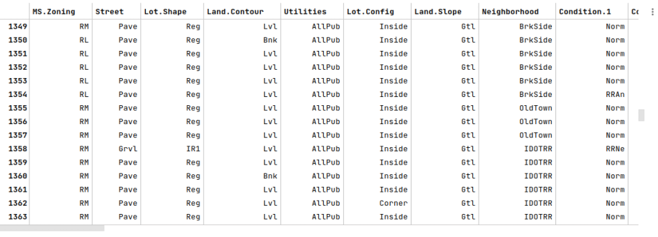
The following illustration shows the few columns/rows of the cleansed housing price dataframe:
The next step is to display the count for all the missing values from the cleansed housing price dataframe as shown below:
home_price_df.isnull().sum()
The following illustration shows the count for all the missing values from the cleansed housing price dataframe:
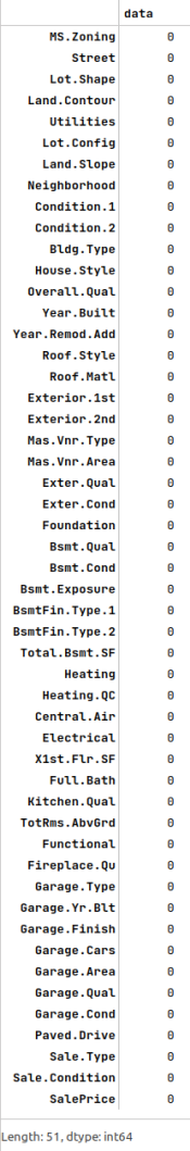
This is to ensure we have no missing values in the cleansed housing price data set.
The next step is to identify and display all the categorical feature variables from the cleansed housing price dataset as shown below:
cat_features = sorted(home_price_df.select_dtypes(include=['object']).columns.tolist())
cat_features
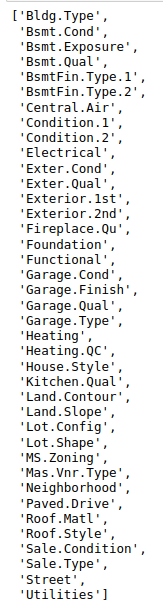
The following illustration shows all the categorical feature variables from the cleansed housing price dataframe:
The next step is to identify all the ordinal features from the above set of categorical feature variables, by cross-checking with the Ames Housing Price - Data Dictionary, and creating a Python dictionary whose keys are the names of the ordinal features and their values are a Python dictionary of the mapping between the labels (of the ordinal feature) to the corresponding numerical values as shown below:
ord_features_dict = {'Bsmt.Cond': {'NA': 0, 'Po': 1, 'Fa': 2, 'TA': 3, 'Gd': 4 , 'Ex': 5},
  'Bsmt.Exposure': {'NA': 0, 'No': 1, 'Mn': 2, 'Av': 3, 'Gd': 4},
  'BsmtFin.Type.1': {'NA': 0, 'Unf': 1, 'LwQ': 2, 'Rec': 3, 'BLQ': 4 , 'ALQ': 5, 'GLQ': 6},
  'BsmtFin.Type.2': {'NA': 0, 'Unf': 1, 'LwQ': 2, 'Rec': 3, 'BLQ': 4 , 'ALQ': 5, 'GLQ': 6},
  'Bsmt.Qual': {'NA': 0, 'Po': 1, 'Fa': 2, 'TA': 3, 'Gd': 4 , 'Ex': 5},
  'Electrical': {'SBrkr': 1, 'FuseA': 2, 'FuseF': 3, 'FuseP': 4, 'Mix': 5},
  'Exter.Cond': {'Po': 1, 'Fa': 2, 'TA': 3, 'Gd': 4 , 'Ex': 5},
  'Exter.Qual': {'Po': 1, 'Fa': 2, 'TA': 3, 'Gd': 4 , 'Ex': 5},
  'Fireplace.Qu': {'NA': 0, 'Po': 1, 'Fa': 2, 'TA': 3, 'Gd': 4 , 'Ex': 5},
  'Functional': {'Sal': 0, 'Sev': 1, 'Maj2': 2, 'Maj1': 3, 'Mod': 4, 'Min2': 5, 'Min1': 6, 'Typ': 7},
  'Garage.Cond': {'NA': 0, 'Po': 1, 'Fa': 2, 'TA': 3, 'Gd': 4 , 'Ex': 5},
  'Garage.Finish': {'NA': 0, 'Unf': 1, 'RFn': 2, 'Fin': 3},
  'Garage.Qual': {'NA': 0, 'Po': 1, 'Fa': 2, 'TA': 3, 'Gd': 4 , 'Ex': 5},
  'Heating.QC': {'Po': 1, 'Fa': 2, 'TA': 3, 'Gd': 4 , 'Ex': 5},
  'Land.Slope': {'Gtl': 1, 'Mod': 2, 'Sev': 3},
  'Lot.Shape': {'Reg': 1, 'IR1': 2, 'IR2': 3, 'IR3': 4},
  'Paved.Drive': {'Y': 1, 'P': 2, 'N': 3},
  'Utilities': {'AllPub': 1, 'NoSewr': 2, 'NoSeWa': 3, 'ELO': 4}
}
For example, consider the ordinal feature Bsmt.Qual. When we transform the labels to numerical values, we will replace all occurences of the label 'NA' with the value 0, the label 'Po' with the value 1, the label 'Fa' with the value 2 and so on.
The next step is to map the categorical labels for each of the ordinal features from the cleansed housing price dataframe into their their numerical representation using the Python dictionary from above as shown below:
home_price_df2 = home_price_df.copy()
for key, val in ord_features_dict.items():
    home_price_df2[key] = home_price_df2[key].map(val)
home_price_df2
The following illustration shows the few columns/rows of the transformed housing price dataframe:
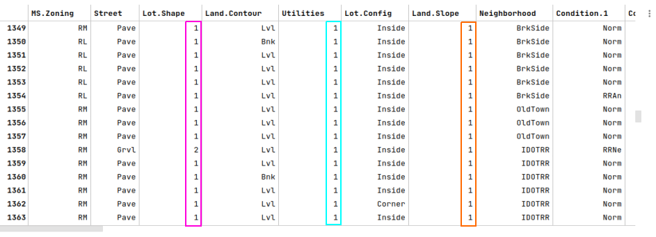
Notice the annotated columns with transformed ordinal feature values - they are all numerical now.
The next step is to identify and collect all the nominal features of the cleansed housing price dataframe as shown below:
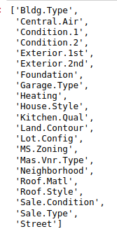
nom_features = [feat for feat in cat_features if feat not in ord_features_dict.keys()]
nom_features
The following illustration displays all the nominal features from the housing price dataframe:
The next step is to create $k-1$ dummy binary variables for each of the nominal feature from the above list using the cleansed housing price dataframe as shown below:
nom_encoded_df = pd.get_dummies(home_price_df[nom_features], prefix_sep='.', drop_first=True, sparse=False)
nom_encoded_df
The following illustration displays the dataframe of all dummy binary variables for each of the nominal features from the cleansed housing price dataframe:
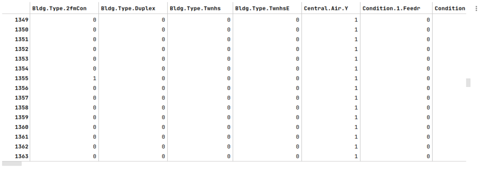
Notice that, with the dummy binary variables generation, we have created about 149 additional features above.
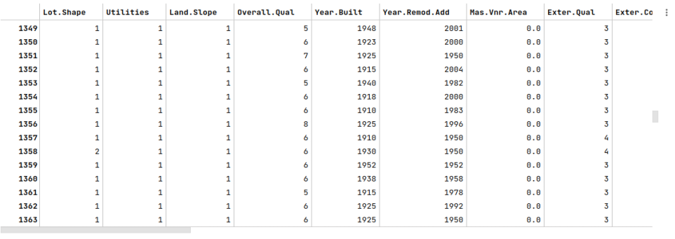
The next step is to drop all the nominal features from the transformed housing price dataframe and display few columns/rows as shown below:
nom_dropped_df = home_price_df2.drop(home_price_df2[nom_features], axis=1)
nom_dropped_df
The following illustration displays few columns/rows from the housing price dataframe:
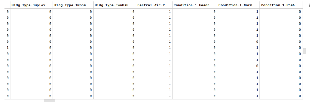
The next step is to merge the dataframe of dummy binary variables we created earlier with the housing price dataframe from above (with dropped nominal features) as shown below:
home_price_df3 = pd.concat([nom_dropped_df, nom_encoded_df], axis=1)
home_price_df3
The following illustration displays few columns/rows from the merged housing price dataframe:
The next step is to display the shape (rows and columns) of the transformed and merged housing price dataframe as shown below:
home_price_df3.shape
The following illustration shows the shape of the transformed and merged housing price dataframe:

Notice the increase in the number of features to 179 after the various transformations.
In the article Regularization using Scikit-Learn - Part 6, we covered the concepts around feature scaling.
The next step is to scale all the features of the transformed and merged housing price dataframe as shown below:
scaler = StandardScaler()
home_price_df3_f = pd.DataFrame(scaler.fit_transform(home_price_df3), columns=home_price_df3.columns, index=home_price_df3.index)
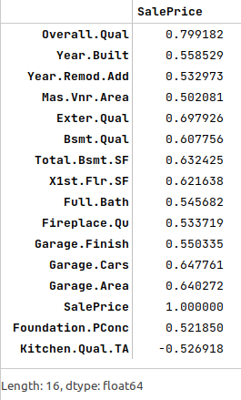
The final step is to display the features from scaled housing price dataframe with a strong correlation to the target feature SalePrice as shown below:
sale_price = home_price_df3_f.corr()['SalePrice']
sale_price[(sale_price >= 0.5) | (sale_price <= -0.5)]
The following illustration displays all the features from scaled housing price dataframe with a strong correlation to the target feature SalePrice:
With this, we wrap the various tasks that are involved in the process of data preparation, before one can get started with the building of the machine learning model.
Hands-on Demo
The following is the link to the Jupyter Notebooks that provides an hands-on demo for this article:
References