Figure.1
| PolarSPARC |
Machine Learning - Regularization using Scikit-Learn - Part 6
| Bhaskar S | 04/22/2022 |
Overview
In Part 5 of this series, we unraveled the concept of Regularization to address model overfitting.
In this part, we get our hands dirty with the different regularization techniques, such as, LASSO, Ridge, and Elastic Net using Scikti-Learn.
Concepts
In this section, we will cover some of the core foundational concepts needed for the hands-on of the various regularization techniques.
Feature Scaling
Scaling of feature variables (or features) is an important step during the exploratory data analysis phase. When the features are in different scales, the features with larger values tend to dominate the regression coefficients and the model gets skewed. Also, the optimization algorithms (to minimize the residual errors) will take longer time to CONVERGE on optimal coefficient values for features with larger values.
Convergence is related to the process of reaching a set goal. The primary goal of Linear Regression (in particular the Ordinary Least Squares method - OLS for short) is to minimize the residual errors to find the line of best fit. But, how does the optimization algorithm work under-the-hood ??? This is where Gradient Descent comes into play. The approach used by Gradient Descent is very similar to that of descending from the top of a mountain to reach the valley at the bottom. Assume, we are at the top of a mountain and the visibility is poor (say, due to fog). How do we start the descend ??? We look around us to find the spot to put our foot to climb down (one step at a time). This process continues till we reach the valley at the bottom (where the slope is minimal). This is exactly how the Gradient Descent algorithm works to find the point with minimal slope by iteratively taking small incremental steps.
In general, there are two commonly used approaches for scaling - first is Normalization and the second is Standardization.
The Normalization scaler takes each feature column $x_i$ to scale its values between $0$ and $1$. In other words, it takes each value of the feature column $x_i$, subtracts from it the minimum value of the feature column $x_{i,min}$, and then divides the result by the range of the feature column $x_{i,max} - x_{i,min}$. This scaler does not change the shape of the original distribution and does not reduce the importance of the outliers.
In mathematical terms:
$\color{red} \boldsymbol{Normalize(x_i)}$ $= \bbox[pink,2pt]{\Large{\frac{x_i - x_{i,min}}{x_{i,max} - x_{i,min}}}}$
The Normalization scalar is sometimes referred to as the Min-Max normalization scaler.
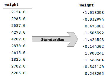
The Standardization scaler takes each feature column $x_i$ to scale its values so that the mean is centered at $0$ with a standard deviation of $1$. In other words, it takes each value of the feature column $x_i$, subtracts from it the mean of the feature column $\mu_{x,i}$, and then divides the result by the standard deviation of the feature column $\sigma_{x,i}$.
In mathematical terms:
$\color{red} \boldsymbol{Standardize(x_i)}$ $= \bbox[pink,2pt]{\Large{\frac{x_i - \mu_{x,i}} {\sigma_{x,i}}}}$
The Standardization scalar is sometimes referred to as the Z-Score normalization scaler.
The following illustration demonstrates the standardization of the feature variable weight from the auto-mpg data set:
Correlation Matrix
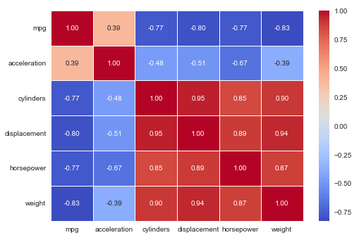
A Correlation Matrix is a square matrix that shows the correlation coefficients between the different feature variables in a data set. The value of $1$ along the main diagonal of the matrix indicates the correlation between a feature variable to itself (hence the perfect score). The correlation matrix is symmetrical with the same set of the correlation coefficients above and below the main diagonal.
The following illustration demonstrates the correlation matrix between different feature variables from the auto-mpg data set:
Variance Inflation Factor
A Variance Inflation Factor (or VIF) is a measure of the amount of multicollinearity present in a set of feature variables. In other words, it measures how much the variance of a regression coefficient for a single feature variable $x_i$ is inflated because of its linear dependence with other feature (or predictor) variables $(x_1, x_2, ..., x_{i-1}, x_{i+1}, ..., x_n)$.
To compute VIF for each feature, pick each feature as the target and perform the multiple regression with all the other features. For each of the multiple regression steps, find the $R^2$ factor and the the VIF is calculated using the formula:
$\color{red} \boldsymbol{VIF_i}$ $= \bbox[pink,2pt]{\Large{\frac{1}{(1 - R_i^2)}}}$
A VIF of $1$ (the minimum possible VIF) means the tested feature is not correlated with the other features, while a large VIF value indicates that the tested feature has linear dependence on the other features. An acceptable range for the VIF value is that it is less than $10$.
Hands-on Regularization
To demonstrate the three regularization techniques, namely LASSO, Ridge, and Elastic Net, we will implement the model that estimates mpg using auto-mpg data set.
The first step is to import all the necessary Python modules such as, matplotlib, pandas, and scikit-learn as shown below:
import numpy as np
import pandas as pd
import matplotlib.pyplot as plt
import seaborn as sns
from statsmodels.stats.outliers_influence import variance_inflation_factor
from sklearn.preprocessing import StandardScaler, PolynomialFeatures
from sklearn.model_selection import train_test_split
from sklearn.linear_model import LinearRegression, Lasso, Ridge, ElasticNet
from sklearn.metrics import mean_squared_error, r2_score
The next step is to load the auto mpg dataset into a pandas dataframe, assign the column names, and perform the tasks to cleanse and prepare the dataset as shown below:
url = 'https://archive.ics.uci.edu/ml/machine-learning-databases/auto-mpg/auto-mpg.data'
auto_df = pd.read_csv(url, delim_whitespace=True)
auto_df.columns = ['mpg', 'cylinders', 'displacement', 'horsepower', 'weight', 'acceleration', 'model_year', 'origin', 'car_name']
auto_df.horsepower = pd.to_numeric(auto_df.horsepower, errors='coerce')
auto_df.car_name = auto_df.car_name.astype('string')
auto_df = auto_df[auto_df.horsepower.notnull()]
auto_df = auto_df[['mpg', 'cylinders', 'displacement', 'horsepower', 'weight', 'acceleration']]
The next step is to create the training dataset and a test dataset with the desired feature (or predictor) variables as shown below:
X_train, X_test, y_train, y_test = train_test_split(auto_df[['mpg', 'acceleration', 'cylinders', 'displacement', 'horsepower', 'weight']], auto_df['mpg'], test_size=0.25, random_state=101)
The next step is to create an instance of the standardization scaler to scale the desired feature (or predictor) variables as shown below:
scaler = StandardScaler()
s_X_train = pd.DataFrame(scaler.fit_transform(X_train), columns=X_train.columns, index=X_train.index)
The following illustration displays the first 10 rows of the pandas dataframe that contains the scaled values of the selected features:
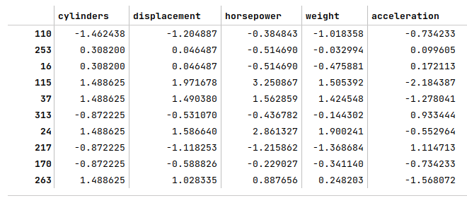
Only the feature variables need to be scaled and *NOT* the target variable
The next step is to display the correlation matrix of the feature (or predictor) variables with the target variable as shown below:
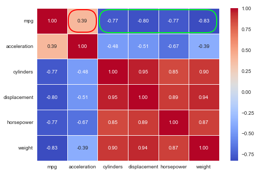
sns.heatmap(s_X_train.corr(), annot=True, cmap='coolwarm', fmt='0.2f', linewidth=0.5)
plt.show()
One can infer from the correlation matrix that the feature acceleration does not have any strong relation with the target variable (annotated in red), while the other features are strongly correlated (annotated in green) as shown in the following illustration:
The next step is to drop the feature acceleration from the scaled training dataset, compute and display the VIF values for the remaining features as shown below:
feature_df = s_X_train.drop(['acceleration', 'mpg'], axis=1)
vif_df = pd.DataFrame()
vif_df['feature_name'] = feature_df.columns
vif_df['vif_value'] = [variance_inflation_factor(feature_df.values, i) for i in range(len(feature_df.columns))]
vif_df
The following illustration displays the VIF values of the scaled selected features:
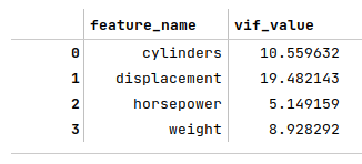
We see the VIF value for the feature displacement is large.
The next step is to drop the feature displacement from the scaled training dataset, re-compute and display the VIF values for the remaining features as shown below:
feature_df = s_X_train.drop('displacement', axis=1)
vif_df = pd.DataFrame()
vif_df['feature_name'] = feature_df.columns
vif_df['vif_value'] = [variance_inflation_factor(feature_df.values, i) for i in range(len(feature_df.columns))]
vif_df
The following illustration displays the recomputed VIF values of the scaled selected features:
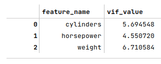
The VIF values for the selected features look much better now.
The next step is to initialize a $3^{rd}$ degree polynomial feature transformer and generate the additional features of the $3^{rd}$ degree using the scaled features as shown below:
transformer = PolynomialFeatures(degree=3, include_bias=True)
s_X_train_f = s_X_train[['cylinders', 'horsepower', 'weight']]
s_X_test_f = s_X_test[['cylinders', 'horsepower', 'weight']]
X_p_train_f = transformer.fit_transform(s_X_train_f)
X_p_test_f = transformer.fit_transform(s_X_test_f)
X_p_train_f.shape
The next step is to initialize and train the polynomial regression model as shown below:
p3_model = LinearRegression()
p3_model.fit(X_p_train_f, y_train)
The next step is to use the trained polynomial regression model to predict the target (mpg) using the test dataset as shown below:
y_predict = p3_model.predict(X_p_test_f)
The next step is to display the $R^2$ value for the polynomial regression model as shown below:
r2_score(y_test, y_predict)
The following illustration displays the $R^2$ value for the model:
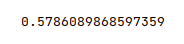
Notice our polynomial regression model performed poorly and achieved an $R^2$ score of about $58\%$ (due to overfitting).
We will now employ the regularization techniques on our $3^{rd}$ degree polynomial features to observe their performance.
We will perform the regularized regression to predict mpg using an aribitrarily determined set of eight values (0.01, 0.5, 1.0, 5.0, 10.0, 20.0, 50.0, 100.0) for the tuning hyperparameter (referred to as $\lambda$ in the mathematical equations in Part 5, specified as alpha in the scikit-learn API).
Before we proceed, the following is the definition of a convenience method to return a Python dictionary from the passed in parameters:
def to_dict(al, sr, r2):
  dc = {'alpha': al}
  for i in range(len(sr)):
      k = "w%02d" % i
      if abs(sr[i]) == 0.00:
          dc[k] = 0.0
      else:
          dc[k] = sr[i]
  dc['R2'] = r2
  return dc
LASSO Regression
The next step is to perform the LASSO regression for the different values of the hyperparamter 'alpha' and display the results as a pandas dataframe as shown below:
rows = []
  for val in [0.01, 0.5, 1.0, 5.0, 10.0, 20.0, 50.0, 100.0]:
      lasso = Lasso(alpha=val)
      lasso.fit(X_p_train_f, y_train)
      y_predict = lasso.predict(X_p_test_f)
      rows.append(to_dict(val, lasso.coef_, r2_score(y_test, y_predict)))
  lasso_df = pd.DataFrame.from_dict(rows)
  with pd.option_context('display.float_format', '{:0.3f}'.format):
      display(lasso_df)
The following illustration displays the results for each iteration of the LASSO regression:
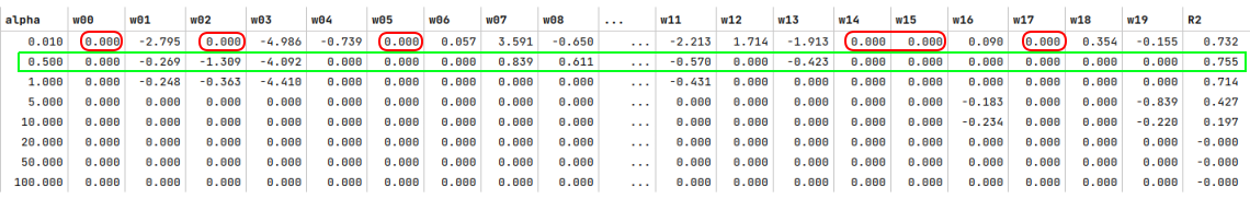
Notice the red rectangles where the regression coefficients for some of the features have become zero. Also, notice the green rectangle that highlights the hyperparameter 'alpha' value for which the $R^2$ score is the highest.
Ridge Regression
The next step is to perform the Ridge regression for the different values of the hyperparamter 'alpha' and display the results as a pandas dataframe as shown below:
rows = []
  for val in [0.01, 0.5, 1.0, 5.0, 10.0, 20.0, 50.0, 100.0]:
      ridge = Ridge(alpha=val)
      ridge.fit(X_p_train_f, y_train)
      y_predict = ridge.predict(X_p_test_f)
      rows.append(to_dict(val, ridge.coef_, r2_score(y_test, y_predict)))
  ridge_df = pd.DataFrame.from_dict(rows)
  with pd.option_context('display.float_format', '{:0.3f}'.format):
      display(ridge_df)
The following illustration displays the results for each iteration of the Ridge regression:
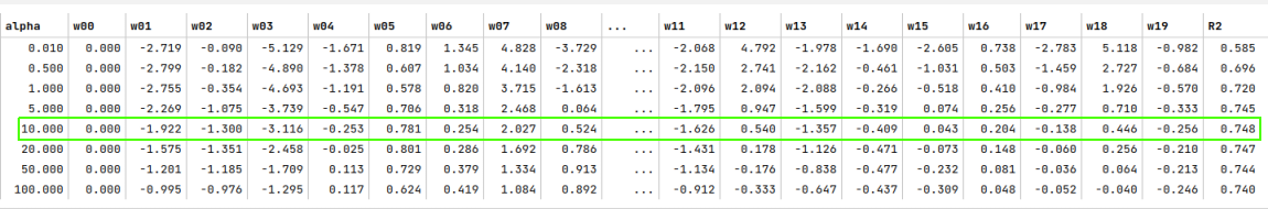
Notice that the regression coefficients of the features never become zero. Also, notice the green rectangle that highlights the hyperparameter 'alpha' value for which the $R^2$ score is the highest.
Elastic Net Regression
The final step is to perform the Elastic Net regression for the different values of the hyperparamter 'alpha' and display the results as a pandas dataframe as shown below:
rows = []
  for val in [0.01, 0.5, 1.0, 5.0, 10.0, 20.0, 50.0, 100.0]:
      elastic = ElasticNet(alpha=val, tol=0.01)
      elastic.fit(X_p_train_f, y_train)
      y_predict = elastic.predict(X_p_test_f)
      rows.append(to_dict(val, elastic.coef_, r2_score(y_test, y_predict)))
  elastic_df = pd.DataFrame.from_dict(rows)
  with pd.option_context('display.float_format', '{:0.3f}'.format):
      display(elastic_df)
The following illustration displays the results for each iteration of the Elastic Net regression:
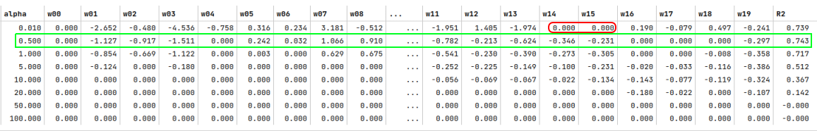
Notice the red rectangles where the regression coefficients for some of the features have become zero. Also, notice the green rectangle that highlights the hyperparameter 'alpha' value for which the $R^2$ score is the highest. In addition, the regression coefficient values are slightly different from that of LASSO or Ridge.
Notice the use of the hyperparameter tol=0.01 in the above case of Elastic Net Regression. This hyperparameter controls at what level of tolerance can the convergence stop during the process of finding the optimal values for the coefficients that minimize the residual errors. Another hyperparameter that can be used is the max_iter. If none specified, one will see the following warning:

ConvergenceWarning: Objective did not converge. You might want to increase the number of iterations, check the scale of the features or consider increasing regularisation.
Hands-on Demo
The following is the link to the Jupyter Notebook that provides an hands-on demo for this article:
References
Machine Learning - Understanding Regularization - Part 5
Machine Learning - Understanding Bias and Variance - Part 4
Machine Learning - Polynomial Regression using Scikit-Learn - Part 3
Machine Learning - Linear Regression using Scikit-Learn - Part 2