Figure.1
| PolarSPARC |
Machine Learning - Understanding Bias and Variance - Part 4
| Bhaskar S | 04/02/2022 |
Overview
In Part 3 of this series, we demonstrated the Polynomial Regression models using Scikit-Learn on the Auto MPG dataset. One of the concepts we touched towards the end was related to overfitting.
Bias and Variance are related to underfitting and overfitting and are essential concepts for developing optimal machine learning models.
We will leverage the dataset Age vs BP to understand bias and variance through practical demonstration.
Bias and Variance
One of the steps in the process of model development involves splitting the known dataset into the training set and the test set. The training set is used to train the model and the test set is used to evaluate the model. In the training phase, the model is learning by finding patterns from the training data, so that it can be used for predicting in the future. There will always be some deviation between what the model predicts versus what is the actual. This is error of estimation from the model. The Bias and Variance are two measures of the error of estimation.
Bias
Bias measures the difference between the actual value versus the estimated value. When the model is simple (as in the case of Simple Linear Regression), the model makes simplistic assumptions and does not attempt to identify all the patterns from the training set, and as a result, the differences (between the estimated and the actual) are large (meaning that the Bias is HIGH). However, when the model is complex (as in the case of Polynomial Regression), the model attempts to capture as many patterns as possible from the training set, and as a result, the differences (between the estimated and the actual) are small (meaning that the Bias is LOW).
In mathematical terms, $Bias = E[(y - \hat{y})]$, where $y$ is the actual value and $\hat{y}$ is the estimated value.
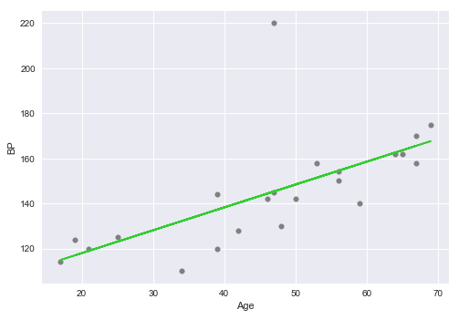
Consider the following plot of the Age vs BP with the line of best fit using Simple Linear Regression:
Contrast the above plot with the following plot of the Age vs BP with the polynomial line of best fit using Polynomial Regression:
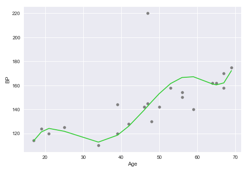
As is evident comparing the above two plots, the Simple Linear Regression model in Figure.1 has a high bias, while the Polynomial Regression model in Figure.2 has a low bias.
Variance
Variance measures the variability in the model estimates between the different training data sets. When the model is simple (as in the case of Simple Linear Regression), the model estimates are consistent between the different training data sets, and as a result, the Variance is LOW. However, when the model is complex (as in the case with Polynomial Regression), the model estimates vary greatly between the different training data sets, and as a result, the Variance is HIGH.
In mathematical terms, $Var(\hat{y}) = E[(\hat{y} - \bar{\hat{y}})^2]$, where $\hat{y}$ is the estimated value and $\bar{\hat{y}}$ is the mean of all the estimated values from different data sets.
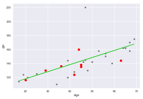
Consider the following plot of the Age vs BP with the line of best fit, along with the training set (in grey) and test set (in red), using Simple Linear Regression:
Contrast the above plot with the following plot of the Age vs BP with the polynomial line of best fit, along with the training set (in grey) and test set (in red), using Polynomial Regression:
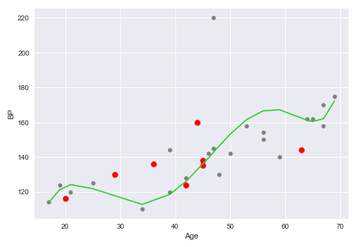
As is evident comparing the above two plots, the Simple Linear Regression model in Figure.3 has a low variance, while the Polynomial Regression model in Figure.4 has a high variance.
Bias-Variance Decomposition
The total error from a model is the sum of two errors - Reducible-Error + Irreducible-Error.
Irreducible-Error is due to various noise and cannot be eliminated, while Reducible-Error is contributed by the bias and the variance components of the model and can be reduced by tuning the model.
In general, the model error is represented using the equation: $Err = Bias^2 + Variance + \varepsilon$.
Let $f(X)$ denote the function that produces the actual target values $Y$ for a given data set $X$. Then, $Y = f(X) + \epsilon$, where $\epsilon$ is the noise.
Also, let $g(X)$ denote the model function that estimates the target values $\hat{Y}$ for the given data set $X$. Then, $\hat{Y} = g(X)$.
From Introduction to Statistics - Part 2, we have learnt the following facts about discrete random variable $X$:
The expected value $E(X) = \bar{X} = \sum_{i=1}^n x_i P(x_i)$ ..... $\color{red} (1)$
The variance $Var(X) = E[(X - \bar{X})^2] = E(X^2) - \bar{X}^2$.
OR, $E(X^2) = \bar{X} + Var(X)$ ..... $\color{red} (2)$
The model error can be expressed as $Err(X) = E[(Y - \hat{Y})^2]$
That is, $Err(X) = E[Y^2 + \hat{Y}^2 - 2 Y \hat{Y}]$
Or, $Err(X) = E[Y^2] + E[\hat{Y}^2] - 2 E[Y] E[\hat{Y}]$ ..... $\color{red} (3)$
From $\color{red} (1)$ and $\color{red} (2)$, we can write $E[Y^2] = \bar{Y}^2 + Var(Y) = E[Y]^2 + Var(Y)$ ..... $\color{red} (4)$
From $\color{red} (1)$ and $\color{red} (2)$, we can write $E[\hat{Y}^2] = \bar{\hat{Y}}^2 + Var(\hat{Y}) = E[\hat{Y}]^2 + Var(\hat{Y})$ ..... $\color{red} (5)$
Replacing $\color{red} (4)$ and $\color{red} (5)$ into $\color{red} (3)$, we get $Err(X) = E[Y]^2 + Var(Y) + E[\hat{Y}]^2 + Var(\hat{Y}) - 2 E[Y] E[\hat{Y}]$
Rearranging the terms, we get $(\color{blue}E[Y]^2 + E[\hat{Y}]^2 - 2 E[Y] E[\hat{Y}]$ $) + Var(\hat{Y}) + Var(Y)$
That is, $Err(X) = E[(Y - \hat{Y})]^2 + Var(\hat{Y}) + Var(f(X) + \epsilon)$ ..... $\color{red} (6)$
For the actual model $f(X)$, there is NO variance and hence $Var(f(X)) = 0$
The variance on noise is a constant. That is, $Var(\epsilon) = \varepsilon$
Rewriting $\color{red} (6)$, we get the following:
$\color{red} \boldsymbol{Err(X)}$ $= \bbox[pink,2pt]{Bias^2 + Var(\hat{Y}) + \varepsilon}$
Bias-Variance Tradeoff
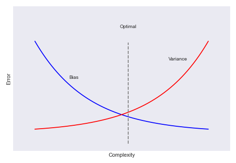
For a given model, there is a tension between the bias and the variance. As the bias increases, the variance decreases and vice-versa. If the model has fewer number of independent feature variables, then the model is simple, resulting in high bias and low variance. On the other hand, if the model has a larger number of independent feature variables, then the model is complex, resulting in low bias and high variance. The goal of Bias-Variance Tradeoff is to find the right balance between the bias and the variance in the model.
The following illustration depicts the bias-variance relationship:
Hands-on Demo
The following is the link to the Jupyter Notebook that provides an hands-on demo for this article:
References
Machine Learning - Polynomial Regression using Scikit-Learn - Part 3
Machine Learning - Linear Regression using Scikit-Learn - Part 2