Figure.1
| PolarSPARC |
Machine Learning - Understanding Regularization - Part 5
| Bhaskar S | 04/15/2022 |
Overview
In Part 4 of this series, we unraveled the concepts related to Bias and Variance and how they relate to underfitting and overfitting.
Overfitting occurs due to the following reasons:
Large number of feature variables (increases model complexity)
Not enough samples for training the model (training data set size is small)
Noise due to collinearity (related features don't expose meaningful relationships)
This is where the techniques of Regularization come in handy to tune (or constrain) the regression coefficients (or weights or parameters) of the regression model to dampen the model variance, thereby controlling model overfitting.
Concepts
In this section, we will cover some of the core concepts, such as covariance, correlation, and norms, as we will referring to them when explaining the regularization techniques.
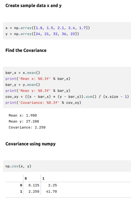
Covariance
The directional measure of linear relationship between two continuous random variables $x$ and $y$ is known as Covariance. The value can be positive (meaning they move in the same direction - if one goes up, the other goes up, and if one goes down, the other goes down) or negative (meaning the move in opposite direction - if one goes up, the other goes down and vice versa).
In mathematical terms:
$\color{red} \boldsymbol{cov(x,y)}$ $= \bbox[pink,2pt]{\Large{\frac{\sum_{i=1}^n (x_i - \bar{x}) (y_i - \bar{y})}{n-1}}}$
The following illustration demonstrates the covariance between two variables:
Covariance only measures the total variation between the two random variables from their expected values and can only indicate the direction of the relationship.
Correlation
The scaled measure of direction as well as the strength of linear relationship between two continuous random variables $x$ and $y$ is known as Correlation (sometimes referred to as the Pearsons Correlation). Correlation which is denoted using $\rho$ builds on covariance by normalizing (rescaling) the variables using their standard deviation.
In mathematical terms:
$\color{red} \boldsymbol{\rho_{(x,y)}}$ $= \bbox[pink,2pt]{\Large{\frac{cov(x,y)}{\sigma_x\sigma_y}}}$
The following illustration demonstrates the correlation between two variables:
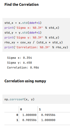
The correlation value is independent of the scale between the two variables (meaning it is standardized) and its value is always between $-1$ and $+1$.
Often times we will hear the term Collinearity, which implies that two feature (or predictor) variables are correlated.
Also, the term Multicollinearity implies that two or more predictor variables are correlated with each other.
Vector Norms
In Introduction to Linear Algebra - Part 1, we covered the basics of vectors and introduced the concept of the vector norm. It is the most common form and is referred to as the L2 Norm (or the Euclidean Norm).
In other words, the L2 Norm (or the Euclidean Norm)is defined as $\lVert \vec{a} \rVert_2 = \sqrt{\sum_{i=1}^n a_{i}^2}$
There is another form of norm called the L1 Norm (or the Manhattan Norm) which is defined as $\lVert \vec{a} \rVert_1 = \sum_{i=1}^n \lvert a_i \rvert$
For example, given the vector $\vec{a} = \begin{bmatrix} 3 \\ -2 \\ 7 \end{bmatrix}$:
The L1 Norm = $3 + (-2) + 7 = 8$.
The L2 Norm = $\sqrt{3^2 + (-2)^2 + 7^2} = \sqrt{9 + 4 + 49} = 7.874$.
Regularization
Regularization is the process of adding a PENALTY term (with a boundary constraint $c$) to the regression error function (SSE) and then minimize the residual errors. This allows one to dampen (or shrink) the regression coefficients $\beta$ towards the boundary constraints $c$ (including zero). This has the effect of increasing the bias, and as a result reducing the variance.
In linear regression, we know the idea is to minimize $E = \sum_{i=1}^n (y_i - (\beta_0 + \beta_1.x_i))^2$ in order to find the best line of fit.
With regularization, the goal is to minimize $E = \sum_{i=1}^n (y_i - (\beta_0 + \beta_1.x_i))^2 + S(\beta)$, where the $S(\beta)$ term is a tunable penalty (or shrinkage) function based on the regression coefficients.
Use regularization only when there are two or more feature (or predictor) variables
To get a hang of regularization better, let us consider a very simple case with one feature variable estimating an outcome variable. The following illustration shows a plot of the regression line of best fit for the hypotetical data set:
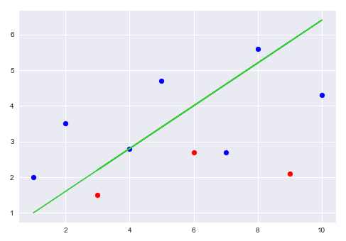
From the illustration above, the blue dots are from the training set and the red dots from a test set (or another training set). The regression line does fit well with the training set but does poorly (large variance) on the test set. The idea of regularization is to add a penalty amount to the residual errors so that the slope (coefficient) is accordingly adjusted (reduced) to compensate for the penalty.
The following illustration shows the original regression line of best fit (green line) for the hypotetical data set with the the regularized (penalized) regression line of best fit (purple line with decreased slope):
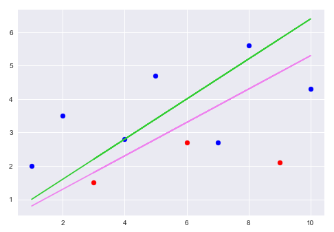
From the illustration above, it is bit more intuitive that the slope of the regularized purple line has decreased (implies the coefficient is reduced), while increasing the bias, and maintaining consistency with respect to variance. This is the fundamental idea behind regularization.
The following are the commonly used regularization techniques:
LASSO
Ridge
Elastic Net
LASSO
LASSO is the abbreviation for Least Absolute Shrinkage and Selection Operator and it uses the L1 norm in combination with a tunable parameter as the penalty or shrinkage term. In other words, $S(\beta) = \lambda \sum_{i=1}^n \lvert a_i \rvert$, where $\lambda$ is the tunable parameter the controls the magnitude or strength of the regularization penalty.
In mathematical terms, $E = \sum_{i=1}^n (y_i - (\beta_0 + \beta_1.x_i))^2 + \lambda \sum_{i=1}^n \lvert a_i \rvert$
Looking at the above error (or cost) function of $E$, as we increase $\lambda$, if we did nothing, then $E$ would increase. However, the goal is to minimize $E$. Intuitively, this means that as $\lambda$ goes up, the regression parameters (or coefficients) have to decrease in order for $E$ to go down.
Linear Regression using this technique is often referred to as LASSO Regression.
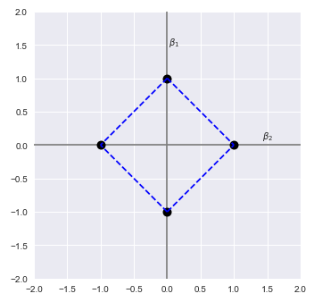
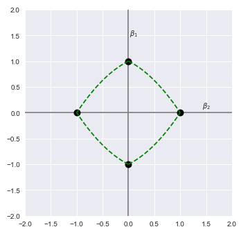
Let us look at it from a geometrical point of view. Let us assume we just have two feature (or predictor) variables and their corresponding coefficients $\beta_1$ and $\beta_2$ (ignore the intercept $\beta_0$ for simplicity).
If we constrain the boundary of the L1 norm to one, meaning $\beta_1 + \beta_2 \le 1$, then following illustration shows the plot of the L1 norm for the coefficients $\beta_1$ and $\beta_2$:
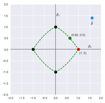
Let $\hat{\beta}$ represent the estimated coefficient values using the least squares line of best fit.
The following illustration shows the plot of the L1 norm for the coefficients $\beta_1$ and $\beta_2$ along with the estimated $\hat{\beta}$:
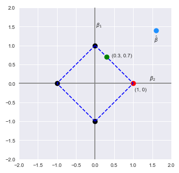
With the LASSO regularization, the idea is to pull the the estimated coefficient values (in cyan color) to be within the constraints of the L1 norm. This means the new estimated coefficient values could either be the green dot or the red dot. As is intuitive, the $\beta$ coefficients will decrease and in fact one of then could also become zero (in the case of the red dot).
As the tunable parameter $\lambda$ is increased, the $\beta$ coefficients that have very low values tend to become zeros. The effect of this behavior is as though we are able to perform FEATURE SELECTION by dropping features that do not add any meaning to the overall outcome (or target) value estimation.
In other words, the LASSO regularization technique only includes feature variables with high coefficient values and tends to drop feature variables with lower coefficient values, which could mean we may be losing some potentially useful feature variables with meaningful relationships.
With the LASSO regularization technique, often times one will hear the term SPARSITY, and this has to do with some of the $\beta$ coefficients becoming exactly zero (sparse vector of $\beta$).
The following are the pros and cons of LASSO regularization technique:
Pros:
Automatic feature selection
Cons:
Ignore some features if the number of features is greater than the data set size
Randomly selects a feature from a group of correlated features
Ridge
Ridge uses the L2 norm in combination with a tunable parameter as the penalty or shrinkage term. In other words, $S(\beta) = \lambda \sum_{i=1}^n a_i^2$, where $\lambda$ is the tunable parameter the controls the magnitude or strength of the regularization penalty.
In mathematical terms, $E = \sum_{i=1}^n (y_i - (\beta_0 + \beta_1.x_i))^2 + \lambda \sum_{i=1}^n a_i^2$
Just like in the case of LASSO technique, as $\lambda$ increases, the regression parameters (or coefficients) will have to decrease in order to minimize $E$. In this case, the penalty term uses the L2 norm (sum of squares of coefficients).
Linear Regression using this technique is often referred to as Ridge Regression.
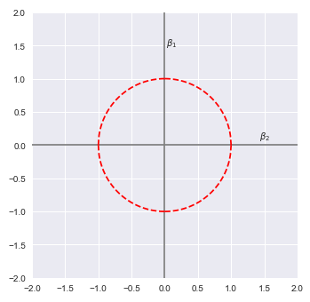
Once again, worth considering a geometrical point of view. Assume we just have two feature (or predictor) variables and their corresponding coefficients $\beta_1$ and $\beta_2$ (ignore the intercept $\beta_0$ for simplicity).
If we constrain the boundary of the L2 norm to one, meaning $\beta_1^2 + \beta_2^2 \le 1$, then following illustration shows the plot of the L2 norm for the coefficients $\beta_1$ and $\beta_2$:
Let $\hat{\beta}$ represent the estimated coefficient values using the least squares line of best fit.
The following illustration shows the plot of the L2 norm for the coefficients $\beta_1$ and $\beta_2$ along with the estimated $\hat{\beta}$:
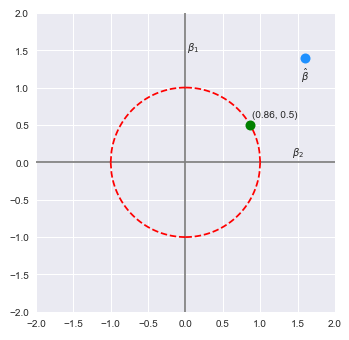
With the Ridge regularization, the idea is to pull the the estimated coefficient values (in cyan color) to be within the constraints of the L2 norm. This means the new estimated coefficient values could be any point within or on the boundary like the example green dot. Like the LASSO technique, as the tunable parameter $\lambda$ is increased, the penalty increases and as a result the $\beta$ coefficients will decrease. However, unlike the LASSO technique, there is a lower probability of making some of the $\beta$ coefficients exactly zero (due to the geometrical boundary of the L2 norm). Instead, they become significantly smaller in value to add any meaningful relationship.
Let us get a mathematical intuition for Ridge regularization. From Part 1 of this series, for regular linear regression, we know the following:
$E = (y^T - \beta^TX^T)(y - X\beta)$
Now, adding the Ridge regularization penalty term, we get the following:
$E = (y^T - \beta^TX^T)(y - X\beta) + \lambda \sum_{i=1}^m \beta_i^2 = (y^T - \beta^TX^T)(y - X\beta) + \lambda \beta^T\beta$
Exapanding the equation, we get: $E = y^Ty - \beta^TX^Ty - y^TX\beta + \beta^TX^TX\beta + \lambda \beta^T\beta$
We know $(y^TX\beta)^T = \beta^TX^Ty$ and $y^TX\beta$ is a scalar. This implies that the transpose of the scalar is the scalar itself. Hence, $y^TX\beta$ can be substituted with $\beta^TX^Ty$.
Therefore, $E = y^Ty - 2\beta^TX^Ty + \beta^TX^TX\beta + \lambda \beta^T\beta = y^Ty - 2\beta^TX^Ty + \beta^TX^TX\beta + \beta^T \lambda \beta = y^Ty - 2\beta^TX^Ty + \beta^TX^TX\beta + \beta^T \lambda I \beta$
That is, $E = y^Ty - 2\beta^TX^Ty + \beta^T (X^TX\beta + \lambda I) \beta$
In order to MINIMIZE the error $E$, we need to take the partial derivatives of the error function with respect to $\beta$ and set the result to zero.
In other words, we need to solve for $\Large{\frac{\partial{E}}{\partial{\beta}}}$ $= 0$.
Therefore, $\Large{\frac{\partial{E}}{\partial{\beta}}}$ $= 0 - 2X^Ty + 2(X^TX\beta + \lambda I)\beta$
That is, $\Large{\frac{\partial{E}}{\partial{\beta}}}$ $= - 2X^Ty + 2(X^TX\beta + \lambda I)\beta$
That is, $- 2X^Ty + 2(X^TX\beta + \lambda I)\beta = 0$
Or, $(X^TX\beta + \lambda I)\beta = X^Ty$
To solve for $\beta$, $(X^TX\beta + \lambda I)^{-1}X^TX\beta = (X^TX\beta + \lambda I)^{-1}X^Ty$
Simplifying, we get the following:
$\color{red} \boldsymbol{\beta}$ $= \bbox[pink,2pt]{(X^TX\beta + \lambda I)^{-1}X^Ty}$
From the above equation, we can infer the fact that, as increase $\lambda$, we decrease the $\beta$.
The following are the pros and cons of Ridge regularization technique:
Pros:
Handles the situation where the number of features is greater than the data set size
Cons:
No capability for feature selection
Elastic Net
Elastic Net is a hybrid regularization technique that uses a combination of both the L1 and the L2 norms as the penalty or shrinkage term. In other words, $S(\beta) = \lambda_1 \sum_{i=1}^n a_i^2 + \lambda_2 \sum_{i=1}^n \lvert a_i \rvert$, where $\lambda_1$ and $\lambda_2$ are the tunable parameters the control the magnitude or strength of the regularization penalty.
In mathematical terms, $E = \sum_{i=1}^n (y_i - (\beta_0 + \beta_1.x_i))^2 + \lambda_1 \sum_{i=1}^n a_i^2 + \lambda_2 \sum_{i=1}^n \lvert a_i \rvert$
The general practice is to choose $\lambda_2 = \alpha$ and $\lambda_1 = \Large{\frac{1 - \alpha}{2}}$, where $\alpha$ is the tunable hyperparameter.
Linear Regression using this technique is often referred to as Elastic Net Regression.
Once again, time to look at it from a geometrical point of view. Assume we just have two feature (or predictor) variables and their corresponding coefficients $\beta_1$ and $\beta_2$ (ignore the intercept $\beta_0$ for simplicity).
If we constrain the boundary of the L2 + L1 norm to one, meaning $(\beta_1^2 + \beta_2^2) + (\beta_1 + \beta_2) \le 1$, then following illustration shows the plot of the L2 + L1 norm for the coefficients $\beta_1$ and $\beta_2$:
Let $\hat{\beta}$ represent the estimated coefficient values using the least squares line of best fit.
The following illustration shows the plot of the L2 + L1 norm for the coefficients $\beta_1$ and $\beta_2$ along with the estimated $\hat{\beta}$:
With the Elastic Net regularization, the idea is to pull the the estimated coefficient values (in cyan color) to be within the constraints of the L2 + L1 norm. Notice the shape of the L2 + L1 norm - it is a combination of L1 norm with the curved sides (from the L2 norm). This means the new estimated coefficient values could either be the green dot or the red dot. Like the LASSO technique, there is a good chance for some of the $\beta$ coefficients to become exactly zero (due to the geometrical boundary of the L2 + L1 norm).
The following are the pros and cons of Elastic Net regularization technique:
Pros:
Automatic feature selection
Handles the situation where the number of features is greater than the data set size
Cons:
Greater computational cost
References
Machine Learning - Understanding Bias and Variance - Part 4
Machine Learning - Polynomial Regression using Scikit-Learn - Part 3
Machine Learning - Linear Regression using Scikit-Learn - Part 2