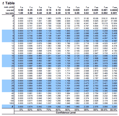
The following illustration shows the T table of the critical values for the commonly used confidence levels and the various degrees of freedom:
T Table
| PolarSPARC |
Introduction to Statistics - Part 4
| Bhaskar S | 07/25/2021 |
In Part 3 of the series, we introduced the concepts around the sampling distribution, the central limit theorem, the point estimation, and the confidence interval.
In this part of the series, we will continue the journey with the point estimation of Population Proportion and the population statistics using the Student's t Distribution, and the Chi-Square Distribution.
Basic Definitions
A Population Proportion is a fraction of the population that has certain characteristics. For example, if we had a population of 1000 people in a remote town and 14 of them owned a store, the population proportion (denoted by p) who own a store is 14 in 1000 or 14/1000.
The Degrees of Freedom (abbreviated as d.f.) is the number of free choices left for computing a sample statistic such as \(\bar{x}\). As an example, consider a classroom with 20 chairs and 20 students. Each of the first 19 students have a choice on which chair to sit on. The 20th student has no freedom of choice. The d.f. for a sample size of n is n - 1.
Estimation for Binomial Distribution
Population Mean and Standard Deviation
From Part 2, we know a binomial distribution is an experiment with n number of trials, where each trial has only two possible outcomes - a success (p for probability of success) or as a failure (q for probability of failure = 1 - p). Tnen, the following is true:
The population mean \(\mu\) can be computed as np
The population standard deviation \(\sigma\) can be computed as \(\sqrt{npq}\)
Estimation of Population Proportion
The point estimate of p (the population proportion of successes) in an experiment where there are x successes in from the n trails is given by the formula: \(\hat{p}\) (pronounced as p-hat) = \(\Large{\frac{x}{n}}\). Then, the population proportion for failures is \(\hat{q} = 1 - \hat{p}\).
If \(n\hat{p} \ge 5\) and \(n\hat{q} \ge 5\), then the margin of error for a given confidence level c can be computed as: E = \(z_c\Large{\sqrt{\frac{\hat{p}\hat{q}}{n}}}\).
The confidence interval for the population proportion p is then \(\hat{p}-E \lt p \lt \hat{p}+E\).
| Example-1 | In a school with 20000 students, 800 students were selected at random to administer a flu shot. Later, it was found that 600 students of select students that were given the shot did not get flu. Find the point estimates for p and q. Also, find the 95% confidence interval for the flu shot to be effective. |
|---|---|
|
Given the sample size n = 800 and the number of successes x = 600. Also, we know \(\hat{p}\) = \(\Large{\frac{x}{n}}\) = \(\Large{\frac{600}{800}}\) = 0.75. Also, \(\hat{q} = 1 - \hat{p}\) = 1 - 0.75 = 0.25. We know the margin of error E = \(z_c\Large{\sqrt{\frac{\hat{p}\hat{q}}{n}}}\). For a confidence level of 95%, \(z_c\) = 1.96. Then, E = \(1.96\Large{\sqrt{\frac{0.75 * 0.25}{800}}}\) \(\approx\) 0.03. That is, \(0.75 - 0.03 \lt p \lt 0.75 + 0.03\) or \(0.72 \lt p \lt 0.78\). Therefore, we can conclude with 95% confidence that the probability for the flu shot to be effective is in the interval 0.72 to 0.78. |
|
Given the margin of error for a confidence level c is E = \(z_c\Large{\sqrt{\frac{\hat{p}\hat{q}}{n}}}\), re-arranging the terms, one can determine the minimum sample size n required to estimate the population proportion as: n = \(\hat{p}\hat{q}\) \(\Large{(\frac{z_c}{E})^2}\).
Estimation for Continuous Distribution
Student's t Distribution
In real-life situations, the population parameter - the standard deviation \(\sigma\) is not known. In these situations, where the sampling distribution for a random variable x is (or almost is) normally distributed OR the sample size is less than 30, one could use the Student's t distribution (also referred to as the t distribution), which has the following properties:
The mean, median, and mode are equal to 0
The distribution is symmetric around the mean
The distribution curve is flatter than the standard normal distribution curve, meaning the curve has a lower height and wider spread (has a larger standard deviation)
The total area under the diatribution curve is 1
As the sample size n increases (\(n \ge 30\)), the distribution approaches the standard normal distribution
The main factor in the distribution is the degree of freedom (represent by d.f.)
The following illustration shows the T table of the critical values for the commonly used confidence levels and the various degrees of freedom:
For a sample distribution of size n, the sample mean \(\bar{x}\) can be computed as \(\bar{x} = \Large{\frac{\Sigma{x}}{n}}\). Also, the sample standard deviation s can be computed as \(s = \Large{\sqrt{\frac{\Sigma{(x - \bar{x})^2}}{n - 1}}}\).
The critical value t for the random variable x that follows a normal distribution with a population mean \(\mu\) can be computed as: t = \(\Large{\frac{\bar{x} - \mu}{s/\sqrt{n}}}\).
The margin of error E for a confidence level c can be computed as: E = \(t_c\Large{\frac{s}{\sqrt{n}}}\).
Given the confidence level of c, the confidence interval for the population parameter \(\mu\) (when the population parameter \(\sigma\) is NOT known) is: \(\bar{x}-E \lt \mu \lt \bar{x}+E\), where E = \(t_c\Large{\frac{s}{\sqrt{n}}}\).
| Example-2 | A sample of 26 same model cars are randomly selected from a car dealership to determine the number of days each car sat on the dealership's lot before it was sold. The sample mean is 9.75 days, with a sample standard deviation of 2.39 days. Construct a 95% confidence interval for the population mean number of days the car model sits on the dealership's lot. |
|---|---|
|
Given the sample size n = 26, the d.f. = n - 1 = 26 - 1 = 25. Also, given the sample mean \(\bar{x}\) = 9.75 and the sample standard deviation s = 2.39. For the confidence level c = 95% and d.f. = 25, we find the critical value \(t_c = 2.060\) from the T table above. The margin of error E = \(t_c\Large{\frac{s}{\sqrt{n}}}\) = \(2.060\Large{\frac{2.39}{\sqrt{26}}}\) = \(2.060\Large{ \frac{2.39}{5.099}}\) \(\approx\) 0.97. We know the confidence interval for the population mean \(\mu\) is \(\bar{x}-E \lt \mu \lt \bar{x}+E\) That is, \(9.75 - 0.97 \lt \mu \lt 9.75 + 0.97\) or \(8.78 \lt \mu \lt 10.72\) Therefore, we can conclude with 95% confidence that the car model sits on the dealership's lot from 8.78 days to 10.72 days |
|
Chi-Square Distribution
The Chi-Square distribution can be used to construct the confidence interval for estimating the variance and the standard deviation, and has the following properties:
The distribution is positively skewed and therefore NOT symmetric
The total area under the diatribution curve is 1
The main factor in the distribution is the degree of freedom (represent by d.f.)
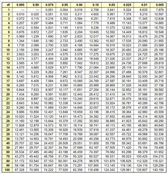
The following illustration shows the Chi-Square table of the critical values for the commonly used confidence levels and the various degrees of freedom:
For a sample distribution of size n, the sample standard deviation s can be computed as \(s = \Large{\sqrt{\frac{\Sigma{(x - \bar{x})^2}}{n - 1}}}\).
The critical value \(\chi^2\) for the random variable x that follows a normal distribution with a population standard deviation \(\sigma\) can be computed as: \(\chi^2\) = \(\Large{\frac{(n - 1)s^2}{\sigma^2}}\).
For a given confidence level c, there are two critical values for this distribution: the right-tail critical value that is denoted by \({\chi_R}^2\) = \(\Large{\frac{1 - c}{2}}\) and the left-tail critical value that is denoted by \({\chi_L}^2\) = \(\Large{\frac{1 + c}{2}}\).
Given the confidence level of c, the confidence interval for the population parameter \(\sigma^2\) is: \(\Large{\frac{(n - 1)s^2}{{\chi_R}^2}}\) \(\lt \sigma^2 \lt\) \(\Large{\frac{(n - 1)s^2}{{\chi_L}^2}}\).
Given the confidence level of c, the confidence interval for the population parameter \(\sigma\) is: \(\Large{\sqrt{\frac{ (n - 1)s^2}{{\chi_R}^2}}}\) \(\lt \sigma \lt\) \(\Large{\sqrt{\frac{(n - 1)s^2}{{\chi_L}^2}}}\).
| Example-3 | A quality control technician randomly selects and weighs 30 samples of an allergy medicine from a manufacturing plant. The sample standard deviation is 1.20 milligrams. Assuming the weights are normally distributed, construct 95% confidence interval for the population standard deviation. |
|---|---|
|
Given the sample size n = 30, the d.f. = n - 1 = 30 - 1 = 29. Also, given the sample standard deviation s = 1.20 milligrams. For the confidence level c = 95%, the area to the right of \({\chi_R}^2\) = \(\Large{\frac{1 - 0.95}{2}}\) = 0.025. For the confidence level c = 95%, the area to the right of \({\chi_L}^2\) = \(\Large{\frac{1 + 0.95}{2}}\) = 0.975. For the confidence level c = 95% and d.f. = 29, we find the critical value for \({\chi_R}^2\) from the Chi-Square table above as 45.722. For the confidence level c = 95% and d.f. = 29, we find the critical value for \({\chi_L}^2\) from the Chi-Square table above as 16.047. We know the confidence interval for the population stanadard deviation \(\sigma\) is \(\Large{\sqrt{\frac{(n - 1)s^2}{ {\chi_R}^2}}}\) \(\lt \sigma \lt\) \(\Large{\sqrt{\frac{(n - 1)s^2}{{\chi_L}^2}}}\). That is, \(\Large{\sqrt{\frac{29 * 1.20}{45.722}}}\) \(\lt \sigma \lt\) \(\Large{\sqrt{\frac{29 * 1.20}{16.047}}}\). Therefore, we can conclude with 95% confidence that the sample weights have a population standard deviation between 0.87 and 1.47 milligrams. |
|
References
Introduction to Statistics - Part 3
Introduction to Statistics - Part 2