Figure.1
| PolarSPARC |
Machine Learning - Gradient Boosting Machine using Scikit-Learn
| Bhaskar S | 07/17/2022 |
Overview
In the article Understanding Ensemble Learning, we covered the concept behind the ensemble method Boosting.
Gradient Boosting Machine (or GBM for short) is one of the machine learning algorithms that leverages an ensemble of weak base models (Decision Trees) for the Boosting method.
In other words, the Gradient Boosting machine learning algorithm iteratively builds a sequence of Decision Trees, such that each of the subsequent Decision Trees work on the residual errors from the preceding trees, to arrive at a robust better predicting model.
Gradient Boosting Machine
In the following sections, we will unravel the steps behind the Gradient Boosting Machine algorithm for regression as well as classification problems.
For a given model $F(x_i)$, the Loss Function $L(y_i, F(x_i))$ would be the Log Likelihood (as was described in the article Logistic Regression) for classification problems and would be the Sum of Squared Errors (as was described in the article Linear Regression) for regression problems.
In addition, the optimization of the Loss Function is performed using the technique of Gradient Descent (as mentioned in the article Regularization). Hence the term Gradient in Gradient Boosting. This implies the use of a Learning Rate coefficient $\gamma$ at each iteration. For our hypothetical usecase, let the Learning Rate $\gamma = 0.1$.
Gradient Boosting Machine for Regression
We will start with the case for a regression problem as it is much easier to get an intuition for how the algorithm works. The Loss Function for regression would then be $L(y_i, F(x_i)) = \sum_{i=1}^N (y_i - \hat{y_i})^2$, where $\hat{y_i} = F(x_i)$. The goal is to minimize the Loss Function. Hence, the residual $r_i = - \Large{\frac{\partial L}{\partial F(x_i)}}$ $= 2(y_i - \hat{y_i})$. Given that $2$ is a constant and will not influence the outcome, we can simplify the residual as $r_i = y_i - \hat{y_i}$.
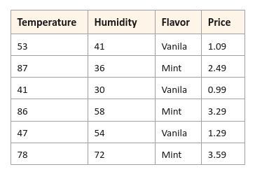
The following illustration displays rows for the hypothetical ice-cream data set:
The following are the steps in the Gradient Boosting algorithm for regression:
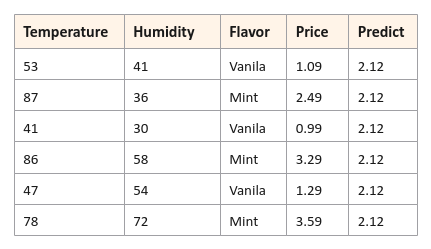
Build a weak base model $F_{m-1}(x_i)$ with just a root node, where $m = 1 ... M$ is the iteration. The predicted value from the weak base model will be the mean $\bar{y}$ of the target (outcome) variable $y_i$ for all the samples from the training data set. For our hypothetical ice-cream data set, we have $6$ samples and hence $\bar{y} = \Large{\frac{1.09+ 2.49+0.99+3.29+1.29+3.59}{6}}$ $= 2.12$ for each sample in the data set as shown below:
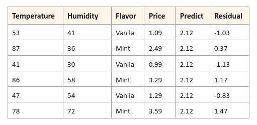
Compute the Residual Errors (referred to as Pseudo Residuals) based on the predictions from the weak base model $F_{m-1}(x_i)$. Mathematically the pseudo residuals are computed as $r_{im} = - \Large{[\frac {\partial L(y_i, F_{m-1}(x_i))}{\partial F_{m-1}(x_i)}]}$ for $i = 1, ..., N$, where $N$ is the number of samples and $m$ is the current iteration. For our data set, the residuals as shown below:
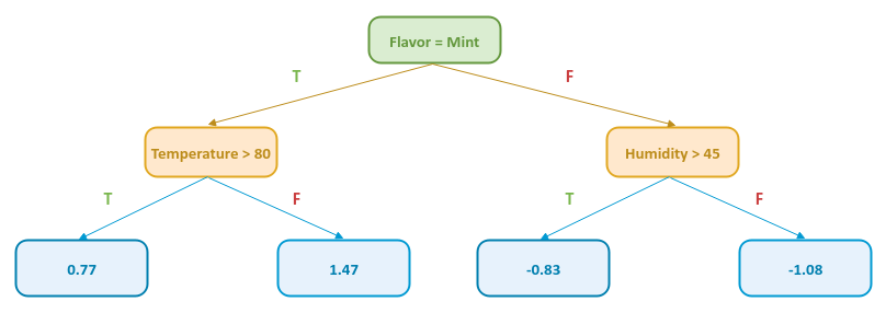
Build a Decision Tree model $H_m(x_i)$ to predict the Residual (target variable) using the feature variables Flavor, Temperature, and Humidity. For our data set, the decision tree could be as shown below:
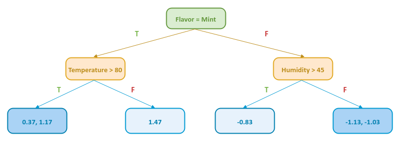
Notice that some of the leaf nodes in the decision tree have multiple values. In those cases, we replace them with their Mean value as shown below:
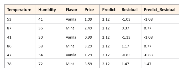
The following illustration indicates the prediction of the residuals from the decision tree model $H_m(x_i)$ above using the features from the hypothetical ice-cream data set:
Update the model by combining the prior model $F_{m-1}(x_i)$ with the current model predicting residuals $H_m(x_i)$ using the Learning Rate $\gamma = 0.1$ as a coefficient. Mathematically this combination is represented as $F_m(x_i) = F_{m-1}(x_i) + \gamma * H_m(x_i)$.
In other words, this means the new target (Price) prediction will be updated using $F_m(x_i) = F_{m-1}(x_i) + \gamma * H_m(x_i)$.
The following illustration shows the samples from the hypothetical ice-cream data set with new target (Price) prediction:
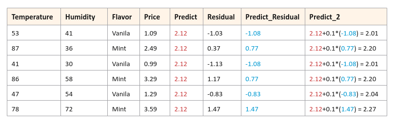
Notice how the newly predicted Prices are tending towards the actual Prices in the hypothetical ice-cream data set.
Go to Step 2 for the next iteration. This process continues until a specified number of models are reached. Note that the iteration will stop early if a perfect prediction state is reached.
Gradient Boosting Machine for Classification
The Loss Function for classification would then be $L(y_i, F(x_i)) = - \sum_{i=1}^N [y_i * log_e(p) + (1 - y_i) * log_e(1 - p)]$, where $p$ is the probability of predicting a class $1$ and $F(x_i)$ predicts the log of odds $log_e \Large{(\frac{p} {1 - p})}$. The goal is to minimize the Loss Function for accurate prediction. Hence, the residual (after simplification of the partial derivative) would be $r_i = - \Large{\frac{\partial L}{\partial F(x_i)}}$ $= y_i - p$.
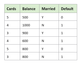
The following illustration displays rows for the hypothetical credit defaults data set:
The following are the steps in the Gradient Boosting algorithm for classification:
Build a weak base model $F_{m-1}(x_i)$ with just a root node, where $m = 1 ... M$ is the iteration. The predicted value from the weak base model will be the probability $P_{m-1}$ of the target (outcome) variable $y_i$ for all the samples in the training data set. The way to get to the probability is through log of odds. In other words $P_{m-1} = \Large{\frac{ e^{ln(odds)}}{1 + e^{ln(odds)}}}$. For our hypothetical credit defaults data set, we have $4$ samples that will default and $2$ that will not and hence $ln(odds) = \Large{\frac{4}{2}}$ $= 0.69$. Therefore, the predicted probability $P_{m-1} = \Large{\frac{e^{0.69}}{1 + e^{0.69}}}$ $= 0.67$ for each sample in the data set as shown below:
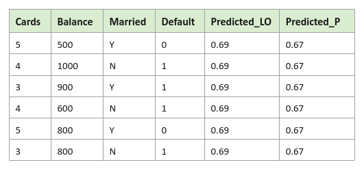
Note we are using the column Predicted_LO for the log of odds and the column Predicted_P for the probabilities.
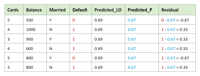
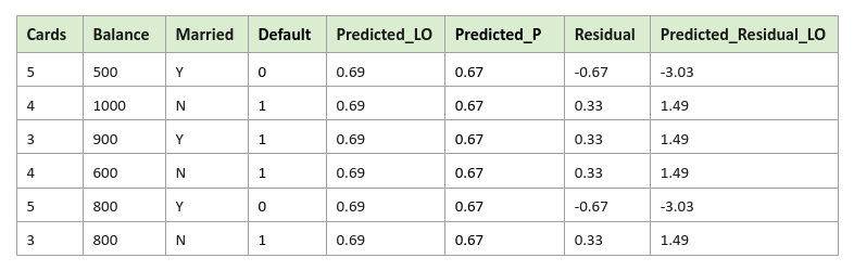
Compute the Residual Errors (referred to as Pseudo Residuals) based on the predictions from the weak base model $F_{m-1}(x_i)$. Mathematically the pseudo residuals are computed as $r_{im} = y_i - p$ for $i = 1, ..., N$, where $N$ is the number of samples and $m$ is the current iteration. For our credit defaults data set, the residuals as shown below:
Build a Decision Tree model $H_m(x_i)$ to predict the Residual (target variable) using the feature variables Married, Cards, and Balance. For our credit defaults data set, the decision tree could be as shown below:
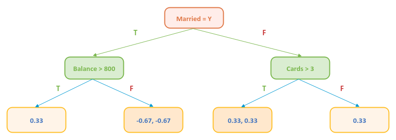
Some of the leaf nodes in the decision tree have multiple values. Given that the values are probabilities, one cannot use their Mean value as was in the case of regression. We will use the formula $\Large{\frac{\sum r_{im}}{\sum P_{m-1} * (1 - P_{m-1})}}$, where $r_{im}$ is the residuals at the leaf and $P_{m-1}$ is the previous probability, to arrive at the log of odds as shown below:
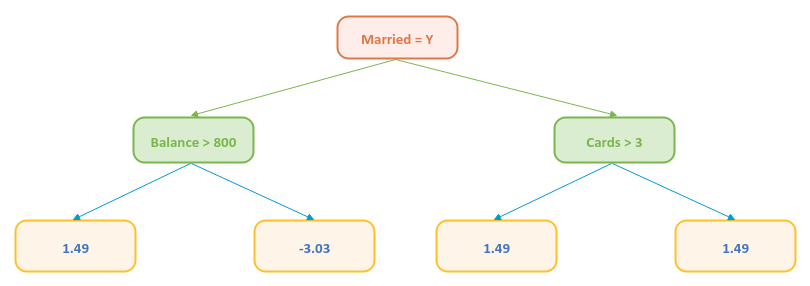
The following illustration indicates the prediction of the residuals (in log odds) from the decision tree model $H_m(x_i)$ above using the features from the credit defaults data set:
Note we are using the column Predicted_Residual_LO for the predicted residuals in log of odds.
Update the model by combining the prior model $F_{m-1}(x_i)$ with the current model predicting residuals $H_m(x_i)$ using the Learning Rate $\gamma = 0.1$ as a coefficient. Mathematically this combination is represented as $F_m(x_i) = F_{m-1}(x_i) + \gamma * H_m(x_i)$.
In other words, this means the new target prediction will be updated using $F_m(x_i) = F_{m-1}(x_i) + \gamma * H_m(x_i)$.
The following illustration shows the samples from the credit defaults data set with new target prediction:
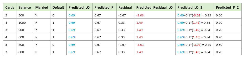
Notice how the newly predicted probabilities are tending towards the actual probabilities in the credit defaults data set.
Go to Step 2 for the next iteration. This process continues until a specified number of models are reached. Note that the iteration will stop early if a perfect prediction state is reached.
Hands-on Demo
In this article, we will use the Diamond Prices data set to demonstrate the use of Gradient Boosting Machine for regression (using scikit-learn) to predict Diamond prices.
The Diamond Prices includes samples with the following features:
carat - denotes the weight of diamond stones in carat unit
color - denotes a factor with levels (D,E,F,G,H,I). D is the highest quality
clarity - denotes a factor with levels (IF,VVS1,VVS2,VS1,VS2). IF is the highest quality
certification - denotes the certification body, a factor with levels ( GIA, IGI, HRD)
The first step is to import all the necessary Python modules such as, pandas and scikit-learn as shown below:
import pandas as pd
from sklearn.model_selection import train_test_split
from sklearn.ensemble import GradientBoostingRegressor
from sklearn.metrics import r2_score
Use the class GradientBoostingClassifier when dealing with classification problems and the class GradientBoostingRegressor when dealing with regression problems.
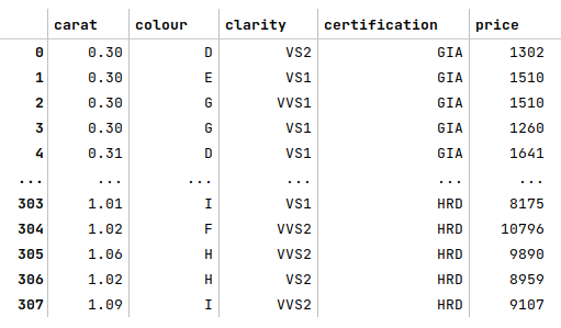
The next step is to load and display the Diamond Prices dataset into a pandas dataframe as shown below:
url = './data/diamond-prices.csv'
diamond_prices_df = pd.read_csv(url, usecols=['carat', 'colour', 'clarity', 'certification', 'price'])
diamond_prices_df
The following illustration shows the few rows of the diamond prices dataframe:
The next step is to identify all the ordinal features from the diamond prices and creating a Python dictionary whose keys are the names of the ordinal features and their values are a Python dictionary of the mapping between the labels (of the ordinal feature) to the corresponding numerical values as shown below:
ord_features_dict = {
  'colour': {'D': 6, 'E': 5, 'F': 4, 'G': 3, 'H': 2 , 'I': 1},
  'clarity': {'IF': 5, 'VVS1': 4, 'VVS2': 3, 'VS1': 2, 'VS2': 1}
}
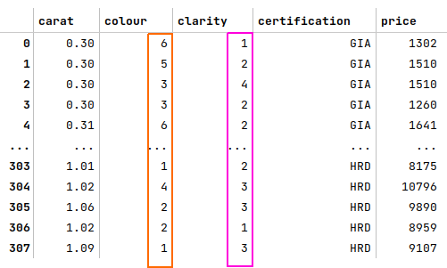
The next step is to map the categorical labels for each of the ordinal features from the diamond prices dataframe into their their numerical representation using the Python dictionary from above as shown below:
for key, val in ord_features_dict.items():
  diamond_prices_df[key] = diamond_prices_df[key].map(val)
diamond_prices_df
The following illustration shows the few rows of the transformed diamond prices dataframe:
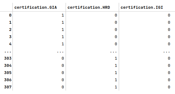
The next step is to create dummy binary variables for the nominal feature 'certification' from the diamond prices data set as shown below:
cert_encoded_df = pd.get_dummies(diamond_prices_df[['certification']], prefix_sep='.', sparse=False)
cert_encoded_df
The following illustration displays the dataframe of all dummy binary variables for the nominal feature 'certification' from the diamond prices dataframe:
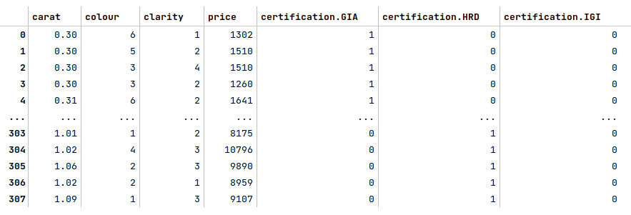
The next step is to drop the nominal feature from the diamond prices dataframe, merge the dataframe of dummy binary variables we created earlier, and display the merged diamond prices dataframe as shown below:
diamond_prices_df = diamond_prices_df.drop('certification', axis=1)
diamond_prices_df = pd.concat([diamond_prices_df, cert_encoded_df], axis=1)
diamond_prices_df
The following illustration displays few rows from the merged diamond prices dataframe:
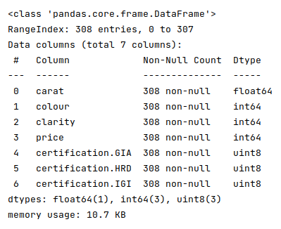
The next step is to display information about the diamond prices dataframe, such as index and column types, memory usage, etc., as shown below:
diamond_prices_df.info()
The following illustration displays information about the diamond prices dataframe:
The next step is to split the diamond prices dataframe into two parts - a training data set and a test data set. The training data set is used to train the ensemble model and the test data set is used to evaluate the ensemble model. In this use case, we split 75% of the samples into the training dataset and remaining 25% into the test dataset as shown below:
X_train, X_test, y_train, y_test = train_test_split(diamond_prices_df, diamond_prices_df['price'], test_size=0.25, random_state=101)
X_train = X_train.drop('price', axis=1)
X_test = X_test.drop('price', axis=1)
The next step is to initialize the Gradient Boosting regression model class from scikit-learn and train the model using the training data set as shown below:
model = GradientBoostingRegressor(max_depth=5, n_estimators=200, learning_rate=0.01, random_state=101)
model.fit(X_train, y_train)
The following are a brief description of some of the hyperparameters used by the AdaBoost model:
max_depth - the maximum depth of each of the decision trees in the ensemble
n_estimators - the total number of trees in the ensemble. The default value is 100
learning_rate - controls the significance for each weak model (decision tree) in the ensemble. The default value is 0.1
The next step is to use the trained model to predict the prices using the test dataset as shown below:
y_predict = model.predict(X_test)
The next step is to display the R2 score for the model performance as shown below:
r2_score(y_test, y_predict)
The following illustration displays the accuracy score for the model performance:
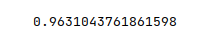
From the above, one can infer that the model seems to predict with great accuracy.
Demo Notebook
The following is the link to the Jupyter Notebook that provides an hands-on demo for this article:
References