PolarSPARC

Introduction to Statistics - Part 6


Bhaskar S 08/15/2021


In Part 5 of the series, we introduced concepts about Hypothesis Testing and explored the One-Mean Z-Test and the One-Mean T-Test.

In this part of the series, we will continue our journey with Hypothesis Testing for Proportions and testing with two samples.

Hypothesis Testing - One Population Proportion

Proportion z-Test

The proportion z-test method a special case of the one-mean z-test and is used to perform a hypothesis test for validating the population proportion.

The following are the requirements for performing a hypothesis test on population proportion with x successes from a fixed n binomial trials:

Let us now solve a problem using the left-tailed test.


Example-1 A mobile service provider claims that less than \(40\%\) of cell phone owners use their phone for most of their online browsing. In a random sample of 100 adults, 31 of them say they use their phone for most of their online browsing. At a significance level of 0.01, is there enough evidence to support the service provider's claim.

Given the population proportion p = 0.40. Therefor, q = 1 - p = 1 - 0.40 = 0.60.

Given the sample size n = 100 with a sample success x = 31. The sample proportion \(\hat{p} = \Large{\frac{x}{n}} = \frac{31}{100}\) = 0.31.

Since np = 0.40 * 100 = 60 and nq = 0.60 * 100 = 60, the sample proportions can be approximated to a normal distribution and we can perform the z-test.

Null hypothesis: \(H_0: p = 0.40\)

Alternate hypothesis: \(H_a: p \lt 0.40\)

In this situation, the hypothesis test is deciding if the population mean is less \(40\%\). Hence, this is a left-tailed test.

We know \(z = \Large{\frac{\hat{p} - p}{\sqrt{pq/n}}}\) = \(\Large{\frac{0.31 - 0.40}{\sqrt{0.40 * 0.60/100}}}\) \(\approx\) -1.84.

For \(\alpha = 0.01\), the critical value from the z-table is \(z_c = -2.33\).

Since the computed standardized test statistic (z) is below the critical value \(z_c\), we FAIL to reject the null hypotesis \(H_0\).

Therefore, at the 0.01 significance level, there is not enough evidence to support the claim that less than \(40\%\) of cell phone owners use their phone for most of their online browsing.

One could also use the p-value to compare against the significance level \(\alpha\) to make a decision. The p-value corresponding to the test statistic z = -1.84 (from the z-table) is \(\approx 0.0329\). Since the p-value is greater than \(\alpha = 0.01\), we FAIL to reject the null hypotesis \(H_0\).


Next, let us now solve a problem using the right-tailed test.


Example-2 The Gallup group conducted a national poll of 1053 U.S. adults that asked their views on an economic stimulus plan. The question was, “As you may know, Congress is considering a new economic stimulus package of at least 800 billion dollars. Do you favor or oppose Congress passing this legislation” Of those sampled, 548 favored passage. At the \(5\%\) significance level, do the data provide sufficient evidence to conclude that a majority more than \(50\%\) of U.S. adults favored passage.

Given the population proportion p = 0.50. Therefor, q = 1 - p = 1 - 0.50 = 0.50.

Given the sample size n = 1053 with a sample success x = 548. The sample proportion \(\hat{p} = \Large{\frac{x}{n}} = \frac{548}{1053}\) = 0.52.

Since np = 0.50 * 1053 = 526.5 and nq = 0.50 * 1053 = 526.5, the sample proportions can be approximated to a normal distribution and we can perform the z-test.

Null hypothesis: \(H_0: p = 0.50\)

Alternate hypothesis: \(H_a: p \gt 0.50\)

In this situation, the hypothesis test is deciding if the population mean is greater \(50\%\). Hence, this is a right-tailed test.

We know \(z = \Large{\frac{\hat{p} - p}{\sqrt{pq/n}}}\) = \(\Large{\frac{0.52 - 0.50}{\sqrt{0.50 * 0.50/1053}}}\) \(\approx\) 1.30.

For \(\alpha = 0.05\), the critical value from the z-table is \(z_c = 1.645\).

Since the computed standardized test statistic (z) is below the critical value \(z_c\), we FAIL to reject the null hypotesis \(H_0\).

Therefore, at the \(5\%\) significance level, the data does not provide sufficient evidence to conclude that the majority of U.S. adults favored the passage of the economic stimulus package.

One could also use the p-value to compare against the significance level \(\alpha\) to make a decision. The p-value corresponding to the test statistic z = 1.30 (from the z-table) is \(\approx 0.0968\). Since the p-value is greater than \(\alpha = 0.05\), we FAIL to reject the null hypotesis \(H_0\).


Finally, let us now solve a problem using the two-tailed test.


Example-3 Based on a survey, \(93\%\) of computer owners believe that they have antivirus programs installed on their computers. In a random sample of 400 scanned computers, it is found that 380 of them actually had the antivirus programs. Use the sample data from the scanned computers to test the claim that 93% of computers have antivirus programs using a \(5\%\) significance level.

Given the population proportion p = 0.93. Therefor, q = 1 - p = 1 - 0.93 = 0.07.

Given the sample size n = 400 with a sample success x = 380. The sample proportion \(\hat{p} = \Large{\frac{x}{n}} = \frac{380}{400}\) = 0.95.

Since np = 0.93 * 400 = 372 and nq = 0.07 * 400 = 28, the sample proportions can be approximated to a normal distribution and we can perform the z-test.

Null hypothesis: \(H_0: p = 0.93\)

Alternate hypothesis: \(H_a: p \ne 0.93\)

In this situation, the hypothesis test is deciding if there is a difference in the claim. Hence, this is a two-tailed test.

We know \(z = \Large{\frac{\hat{p} - p}{\sqrt{pq/n}}}\) = \(\Large{\frac{0.95 - 0.93}{\sqrt{0.93 * 0.07/400}}}\) \(\approx\) 1.57.

For \(\alpha = 0.05\), the critical values from the z-table for -0.025 and 0.025 (since it is a two-tailed test) are \(z_c = -1.96\) and \(z_c = 1.96\).

Since the computed standardized test statistic (z) is below the critical values \(z_c = 1.96\) and \(z_c = -1.96\), we FAIL to reject the null hypotesis \(H_0\).

Therefore, at the \(5\%\) significance level, the data does not provide sufficient evidence to warrant the rejection of the claim that 93% of computers have antivirus programs.

One could also use the p-value to compare against the significance level \(\alpha\) to make a decision. The p-value corresponding to the test statistic z = 1.57 (from the z-table) is \(\approx 0.0582\). Since this is a two-tailed test, the p-value is 2 times the probability, which is \(\approx 0.1164\). Since the p-value is greater than \(\alpha = 0.05\), we FAIL to reject the null hypotesis \(H_0\).


Hypothesis Testing - Two Population Means

Often times, we conduct hypothesis tests to determine differences between two populations. In the following section(s), we will use the following notation:

Independent Samples - Two-Means z-Test

The two-means z-test method is used to compare the means of two independent samples and determine if they came from the same population and that the population means are equal. The following are some of the requirements for performing the two-means z-test:

When the above conditions are satisfied, the following are the steps to perform the two-means z-test:

Let us now solve a problem for the two-means z-test.


Example-4 A student is asked to compare the average heights of two groups. The first group consists of individuals of Italian nationality with the following heights: 174, 168, 180, 175, 169, 181, 175, 168, 179, 174, 182, 174, 169, 177, and 182 respectively. The second group consists of individuals of German nationality with the following heights: 175, 169, 173, 188, 173, 186, 175, 185, 174, 179, 180, 179, 176, and 180 respectively. The standard deviation of the Italian population is 5 and the standard deviation of the German population is 6.5. With a \(95\%\) confidence level, determine if there any difference in the average heights of two groups.

The two sample sizes are \(n_1 = 15\) and \(n_2 = 14\). Given sample sizes are \(\lt 30\), so we need to determine if the two samples are normally distributed.

One can use the Q-Q plot to determine a a data set is normally distributed. A Q-Q (short for 'quantile-quantile') plot is often used to determine whether or not a set of data follows a normal distribution. The x-axis of the Q-Q plot displays the theoretical quantiles, while the y-axis of the Q-Q plot displays the actual data set. If the data values fall along a roughly straight line at a 45-degree angle, then the data is normally distributed.

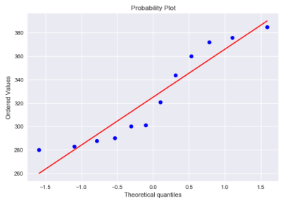
The following illustration shows the distribution of the heights for the first group consisting of Italian nationality:


Italian Distribution
Heights of Italians

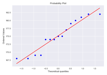
The distribution for the first group consisting of Italian nationality is almost normal.

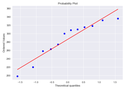
The following illustration shows the distribution of the heights for the second group consisting of German nationality:


German Distribution
Heights of Germans

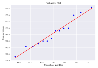
The distribution for the second group consisting of German nationality is almost normal.

The sample mean \(\bar{x_1}\) for the first group is computed by adding all the sample heights of the Italians and dividing by \(n_1 = 15\). That is, \(\bar{x_1} \approx 175.13\).

The sample mean \(\bar{x_2}\) for the second group is computed by adding all the sample heights of the Germans and dividing by \(n_2 = 14\). That is, \(\bar{x_2} = 178.0\).

Null hypothesis: \(H_0: \mu_1 = \mu_2\)

Alternate hypothesis: \(H_a: \mu_1 \ne \mu_2\)

In this situation, the hypothesis test is deciding if there is a difference between the mean heights of the two groups. Hence, this is a two-tailed test.

Given the confidence level \(c = 95\%\), significance level \(\alpha = (1 - c) = 0.05\). Also, given are the population standard deviation of the two groups \(\sigma_1 = 5\) and \(\sigma_2 = 6.5\) respectively.

We know \(\sigma_{\bar{x_1}-\bar{x_2}}\) = \(\Large{\sqrt{\frac{\sigma_1^2}{n_1} + \frac{\sigma_2^2}{n_2}}}\) = \(\Large{\sqrt{\frac{5^2}{15} + \frac{6.5^2}{14}}}\) \(\approx 2.164\).

Also, we know z = \(\Large{\frac{\bar{x_1} - \bar{x_2}}{\sigma_{\bar{x_1}-\bar{x_2}}}}\) = \(\Large{\frac{175.13 - 178.0}{2.164}}\) \(\approx\) -1.324.

For \(\alpha = 0.05\), the critical values from the z-table for -0.025 and 0.025 (since it is a two-tailed test) are \(z_c = -1.96\) and \(z_c = 1.96\).

Since the computed standardized test statistic (z) is below the critical values \(z_c = -1.96\), we FAIL to reject the null hypotesis \(H_0\).

Therefore, with the \(95\%\) confidence level, we conclude that the means heights of the two groups are NOT significantly different.

One could also use the p-value to compare against the significance level \(\alpha\) to make a decision. The p-value corresponding to the test statistic z = -1.324 (from the z-table) is \(\approx 0.0927\). Since this is a two-tailed test, the p-value is 2 times the probability, which is \(\approx 0.1853\). Since the p-value is greater than \(\alpha = 0.05\), we FAIL to reject the null hypotesis \(H_0\).


Independent Samples - Two-Means t-Test

In reality, one would not know the standard deviation of the population. That is when the two-means t-test method is used to compare the means of two independent samples and determine if they came from the same population and that the population means are equal. The following are some of the requirements for performing the two-means t-test:

When the above conditions are satisfied, the following are the steps to perform the two-means t-test:

Let us now solve a problem for the two-means t-test.


Example-5 A new software technology is developed to help data analysts reduce the time required to analaze and generate reports. A random sample of 24 data analysts are selected such that 12 of the data analysts are instructed to produce reports using the current technology, while the other 12 data analysts are instructed to produce reports using the newer technology. The researcher in charge of the new software technology evaluation hopes to show that the new software technology will provide a shorter mean completion time. The following are the mean completion times using the current technology: 300, 280, 344, 385, 372, 360, 288, 321, 376, 290, 301, and 283 respectively. The following are the mean completion times using the new software technology: 274, 220, 308, 336, 198, 300, 315, 258, 318, 310, 332, and 263 respectively. Use a significance level \(\alpha = 0.05\) to verify the claim.

The two sample sizes are \(n_1 = 12\) and \(n_2 = 12\). Given sample sizes are \(\lt 30\), so we need to determine if the two samples are normally distributed.

One can use the Q-Q plot to determine a a data set is normally distributed.

The following illustration shows the distribution of the mean completion times for the current technology:


Current Technology
Current Technology

The distribution for the current technology is almost normal.

The following illustration shows the distribution of the mean completion times for the new software technology:


New Software Technology

The distribution for the new software technology is almost normal.

The sample mean \(\bar{x_1}\) for the first sample is computed by adding all the mean completion times for the current technology and dividing by \(n_1 = 12\). That is, \(\bar{x_1} = 325.0\).

The sample mean \(\bar{x_2}\) for the second sample is computed by adding all the mean completion times for the new software technology and dividing by \(n_2 = 12\). That is, \(\bar{x_2} = 286.0\).

The sample standard deviation \(s_1 = \Large{\sqrt{\frac{\Sigma{(x - \bar{x_1})^2}}{n_1 - 1}}}\) = 39.995.

The sample standard deviation \(s_2 = \Large{\sqrt{\frac{\Sigma{(x - \bar{x_2})^2}}{n_2 - 1}}}\) = 43.998.

Null hypothesis: \(H_0: \mu_1 = \mu_2\)

Alternate hypothesis: \(H_a: \mu_1 \gt \mu_2\)

In this situation, the hypothesis test is deciding if the mean completion time of current technology is greater than the mean completion time of new software technology. Hence, this is a right-tailed test.

Given the significance level \(\alpha = 0.05\).

We know \(s_{\bar{x_1}-\bar{x_2}}\) = \(\Large{\sqrt{\frac{s_1^2}{n_1} + \frac{s_2^2}{n_2}}}\) = \(\Large{\sqrt{\frac{39.995^2}{12} + \frac{43.998^2}{12}}}\) \(\approx 17.165\).

Also, we know t = \(\Large{\frac{\bar{x_1} - \bar{x_2}}{s_{\bar{x_1}-\bar{x_2}}}}\) = \(\Large{\frac{325.0 - 286.0}{17.165}}\) \(\approx\) 2.272.

We know d.f. = \(\Large{\frac{(\frac{s_1^2}{n_1} + \frac{s_2^2}{n_2})}{\frac{1}{n_1 - 1}{[\frac{s_1^2}{n_1}]}^2 + \frac{1}{n_2 - 1}{[\frac{s_2^2}{n_2}]}^2}}\) \(\approx 22\)

For \(\alpha = 0.05\), the critical value from the t-table for d.f. = 22 is \(t_c \approx 1.717\).

Since the computed standardized test statistic (t) is beyond the critical value \(t_c\), we REJECT the null hypotesis \(H_0\).

Therefore, at the 0.05 significance level, the sample data provides sufficient evidence to conclude that the mean completion times for the new software technology is lesser then the current technology.

One could also use the p-value to compare against the significance level \(\alpha\) and degrees of freedom (d.f.) to make a decision. The p-value corresponding to the test statistic t = 2.272 (from the t-table) is \(\approx 0.0166\). Since the p-value is less than \(\alpha = 0.05\), we can REJECT the null hypotesis \(H_0\).


References

Introduction to Statistics - Part 5

Introduction to Statistics - Part 4

Introduction to Statistics - Part 3

Introduction to Statistics - Part 2

Introduction to Statistics - Part 1

Introduction to Probability

Introduction to Permutation & Combinations


© PolarSPARC