Deep Learning - Bidirectional Recurrent Neural Network

Bhaskar S

09/16/2023

Introduction

In the previous article Recurrent Neural Network of this series, we provided an explanation of the inner workings and a practical demo of RNN for the restaurant reviews sentiment prediction.

The typical RNN model processes a sequence of text tokens in the forward direction (that is from the first to the last) at each time step during training and later during prediction.

In other words, the typical RNN model looks at the text token at the current time step and the text tokens from the past time steps (via the hidden state) to train and later to predict.

The RNN model could learn better if the model could also see the text tokens from the future time step.

For example consider the following sentences:

$The\;food\;was\;not\;\textbf{bad}$

and

$The\;food\;was\;not\;\textbf{good}$

As is evident from the two sentences above, the sentiment of the sentences above can be determined only after seeing the last word from the sentences.

This is where the Bidirectional Recurrent Neural Network comes into play, which looks at both the past and the future text tokens to learn and predict better.

Bidirectional Recurrent Neural Network

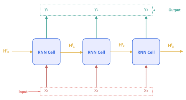
The following illustration shows the typical Recurrent Neural Network unfolded over time for $3$ input tokens $x_1, x_2, x_3$:

Figure.1

Note that the parameters $H^f_0$ through $H^f_3$ are the hidden states which captures the historical sequence of input tokens going in the forward direction.

The following illustration shows the high-level view of a Bidirectional Recurrent Neural Network:

Figure.2

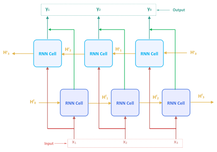
As can be inferred from Figure.2 above, the Bidirectional RNN model is nothing more than two independent RNN models - one processing input tokens from first to last and the other processing input tokens in the reverse order from last to first.

The parameters $H^f_0$ through $H^f_3$ are the hidden states associated with the forward processing RNN model, while the parameters $H^r_0$ through $H^r_3$ are the hidden states associated with the backward processing RNN model.

$y_1$ through $y_3$ are the outputs from the Bidirectional RNN model, each of which is a concatenation of the corresponding outputs from the two independent RNN models.

Hands-on Bidirectional RNN Using PyTorch

To perform sentiment analysis using the Bidirectional RNN model, we will be leveraging the Restaurant Reviews data set from Kaggle.

To import the necessary Python module(s), execute the following code snippet:

import numpy as np
import pandas as pd
import nltk
import torch
from collections import Counter
from nltk.corpus import stopwords
from nltk.tokenize import WordPunctTokenizer
from sklearn.model_selection import train_test_split
from torch import nn
from torchmetrics import Accuracy

Assuming the logged in user is alice, to set the correct path to the nltk data packages, execute the following code snippet:

nltk.data.path.append("/home/alice/nltk_data")

Download the Kaggle Restaurant Reviews data set to the directory /home/alice/txt_data.

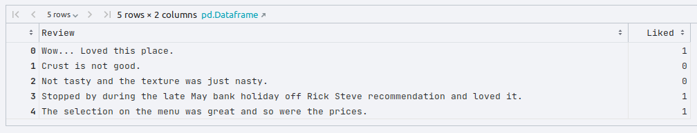
To load the tab-separated restaurant reviews data set into pandas and display the first few rows, execute the following code snippet:

reviews_df = pd.read_csv('./txt_data/Restaurant_Reviews.tsv', sep='\t')
reviews_df.head()

The following would be a typical output:

Figure.3

To create an instance of the stop words, the word tokenizer, and the lemmatizer, execute the following code snippet:

stop_words = stopwords.words('english')
word_tokenizer = WordPunctTokenizer()
word_lemmatizer = nltk.WordNetLemmatizer()

To extract all the text reviews as a list of sentences (corpus), execute the following code snippet:

reviews_txt = reviews_df.Review.values.tolist()

To cleanse the sentences from the corpus by removing the punctuations, stop words, two-letter words, converting words to their roots, collecting all the unique words from the reviews corpus, execute the following code snippet:

vocabulary_counter = Counter()
cleansed_review_txt = []
for review in reviews_txt:
  tokens = word_tokenizer.tokenize(review)
  alpha_words = [word.lower() for word in tokens if word.isalpha() and len(word) > 2 and word not in stop_words]
  final_words = [word_lemmatizer.lemmatize(word) for word in alpha_words]
  vocabulary_counter.update(final_words)
  cleansed_review = ' '.join(final_words)
  cleansed_review_txt.append(cleansed_review)

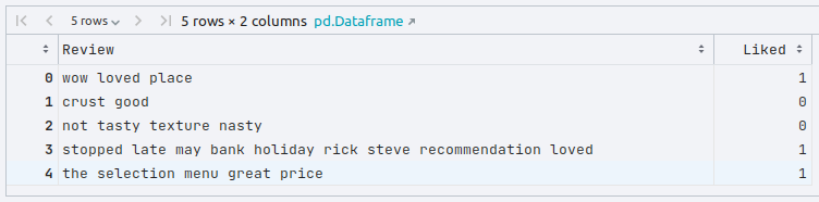
To update the original reviews in the reviews pandas dataframe with the cleansed restaurant reviews display the first few rows, execute the following code snippet:

reviews_df['Review'] = cleansed_review_txt
reviews_df.head()

The following would be a typical output:

Figure.4

We need an index position for each word in the corpus. For this demonstration, we will use $500$ of the most common words. To create a word to index dictionary for the most common words, execute the following code snippet:

one_hot_size = 500
common_vocabulary = vocabulary_counter.most_common(one_hot_size)
word_to_index = {word:idx for idx, (word, count) in enumerate(common_vocabulary)}

We will use the word to index dictionary from above to convert each of the restaurant reviews (in text form) to a one-hot encoded vector (of numbers - ones for word present or zeros for absent). To create a list of one-hot encoded vector for each of the reviews, execute the following code snippet:

clean_reviews_txt = reviews_df.Review.values.tolist()
clean_reviews_labels = reviews_df.Liked.values.tolist()
one_hot_reviews_list = []
for review in clean_reviews_txt:
  tokens = word_tokenizer.tokenize(review)
  one_hot_review = np.zeros((one_hot_size), dtype=np.float32)
  for word in tokens:
    if word in word_to_index:
      one_hot_review[word_to_index[word]] = 1
  one_hot_reviews_list.append(one_hot_review)

To create the tensor objects for the input and the corresponding labels, execute the following code snippet:

X = torch.tensor(np.array(one_hot_reviews_list), dtype=torch.float)
y = torch.tensor(np.array(clean_reviews_labels), dtype=torch.float).unsqueeze(dim=1)

To create the training and testing data sets, execute the following code snippet:

X_train, X_test, y_train, y_test = train_test_split(X, y, test_size=0.2, random_state=101)

To initialize variables for the number of input features, the size of the hidden state, number of hidden layers and the number of outputs, execute the following code snippet:

input_size = one_hot_size
hidden_size = 32
no_layers = 2
output_size = 1

To create a Bidirectional RNN model for the reviews sentiment analysis using a single hidden layer, execute the following code snippet:

class SentimentalBiRNN(nn.Module):
  def __init__(self, input_sz, hidden_sz, output_sz):
    super(SentimentalBiRNN, self).__init__()
    self.rnn = nn.RNN(input_size=input_sz, hidden_size=hidden_sz, num_layers=no_layers, bidirectional=True)
    self.linear = nn.Linear(hidden_size*2, output_sz) # hidden_state*2 for bidirectional

  def forward(self, x_in: torch.Tensor):
    output, _ = self.rnn(x_in)
    output = self.linear(output)
    return output

To create an instance of the SentimentalBiRNN model, execute the following code snippet:

snt_model = SentimentalBiRNN(input_size, hidden_size, output_size)

Since the sentiments can either be positive or negative (binary), we will create an instance of the Binary Cross Entropy loss function by executing the following code snippet:

criterion = nn.BCEWithLogitsLoss()

Note that the BCEWithLogitsLoss loss function combines both the sigmoid activation function and the binary cross entropy loss function into a single function.

To create an instance of the gradient descent function, execute the following code snippet:

optimizer = torch.optim.Adam(snt_model.parameters(), lr=0.05)

To implement the iterative training loop for the forward pass to predict, compute the loss, and execute the backward pass to adjust the parameters, execute the following code snippet:

num_epochs = 1001
for epoch in range(1, num_epochs):
  snt_model.train()
  optimizer.zero_grad()
  y_predict = snt_model(X_train)
  loss = criterion(y_predict, y_train)
  if epoch % 100 == 0:
    print(f'Sentiment Model RNN (Bidirectional) -> Epoch: {epoch}, Loss: {loss}')
  loss.backward()
  optimizer.step()

The following would be a typical output:

Output.1

Sentiment Model RNN (Bidirectional) -> Epoch: 10, Loss: 0.613365888595581
Sentiment Model RNN (Bidirectional) -> Epoch: 20, Loss: 0.4955539405345917
Sentiment Model RNN (Bidirectional) -> Epoch: 30, Loss: 0.46131765842437744
Sentiment Model RNN (Bidirectional) -> Epoch: 40, Loss: 0.3915174901485443
Sentiment Model RNN (Bidirectional) -> Epoch: 50, Loss: 0.3410133123397827
Sentiment Model RNN (Bidirectional) -> Epoch: 60, Loss: 0.21461406350135803
Sentiment Model RNN (Bidirectional) -> Epoch: 70, Loss: 0.14015011489391327
Sentiment Model RNN (Bidirectional) -> Epoch: 80, Loss: 0.08907901495695114
Sentiment Model RNN (Bidirectional) -> Epoch: 90, Loss: 0.029370827600359917
Sentiment Model RNN (Bidirectional) -> Epoch: 100, Loss: 0.011738807894289494

To predict the target values using the trained model, execute the following code snippet:

snt_model.eval()
with torch.no_grad():
  y_predict, _ = snt_model(X_test)
  y_predict = torch.round(y_predict)

To display the model prediction accuracy, execute the following code snippet:

accuracy = Accuracy(task='binary', num_classes=2)

print(f'Sentiment Model RNN (Bidirectional) -> Accuracy: {accuracy(y_predict, y_test)}')

The following would be a typical output:

Output.2

Sentiment Model RNN (Bidirectional) -> Accuracy: 0.7649999856948853

This concludes the explanation and demonstration of the Bidirectional Recurrent Neural Network model.

References

PyTorch Documentation

Deep Learning - Recurrent Neural Network

Deep Learning - The Vanishing Gradient

Introduction to Deep Learning - Part 7

Introduction to Deep Learning - Part 6

Introduction to Deep Learning - Part 5

Introduction to Deep Learning - Part 4

Introduction to Deep Learning - Part 3

Introduction to Deep Learning - Part 2

Introduction to Deep Learning - Part 1